ULC405 Tutorial Companion

Start here

The one idea behind the whole course

A transmission line is four numbers pretending to be a wire: resistance (it heats up), inductance (current makes a magnetic field), capacitance (voltage makes an electric field) and conductance (leakage, usually ignored). Every problem on these seven sheets is either find one of those four numbers from the geometry, or the line is a physical object that must not fall down, flash over, or cost too much.

That split is worth holding onto, because it tells you which formula sheet you are in before you read a single number. Sheets 1–3 are money. Sheet 4 is the four parameters. Sheets 5–7 are the line as hardware: how much it sags, how its insulators share voltage, and what happens when you bury it.

Three habits that fix most wrong answers

Decide per-phase or three-phase, once, in writing. A three-phase quantity is stated line-to-line; nearly every formula wants line-to-neutral, which is smaller by √3. Write V_ph = V_L/√3 at the top of the page and never think about it again.
Convert to metres and metres. Diameters arrive in cm and mm, spacings in m, lengths in km. Inductance and capacitance formulas are per metre and take a ratio — so both distances in the ratio must share a unit, and the answer gets multiplied by length at the end.
Ask whether the stated voltage is rms or peak. Insulator and cable questions quietly switch to peak, and the factor √2 is the difference between their printed answer and yours. Two problems on these sheets turn on exactly this.

Two topics your material does not contain

The per-unit system (Sheet 2) is not in the six unit decks. It is in Wadhwa §1.5, "The Per Unit System" — pdf p26, chapter 1. Everything you need is in Sheet 2 below anyway.

Kelvin's law (Sheet 3) appears in neither the decks nor Wadhwa. The only "Kelvin" in either is Lord Kelvin's method of images, which is a capacitance technique and a different thing entirely. Sheet 3 below derives the law from scratch; both of its printed answers check out, so the derivation is sound even though the source is missing.

Theory first Read once, then the sheets make sense

Where all seven sheets come from

Six ideas, each one paragraph of physics and one formula. Every problem you have been set is one of these six ideas with numbers attached — knowing which one you are in is most of the work.

A power system exists to move energy from where it is generated to where it is used, and almost every design decision in it is a fight against two enemies: I²R heating, which wastes the energy you are trying to sell, and electric field strength, which destroys the insulation you are trying to keep. Sheets 1–4 are the first enemy. Sheets 5–7 are the second. That is the whole course.

1 · Why everything is transmitted at high voltage

To deliver a fixed power P you can send a big current at low voltage or a small current at high voltage, because P = VI cosθ. But the loss is W = I²R — it follows the current, not the power. Halve the current and you quarter the loss. So for a fixed acceptable loss you can use a quarter of the copper, and the conductor volume comes out as

Volume of conductor material v = P²ρl²W V² cos²θ

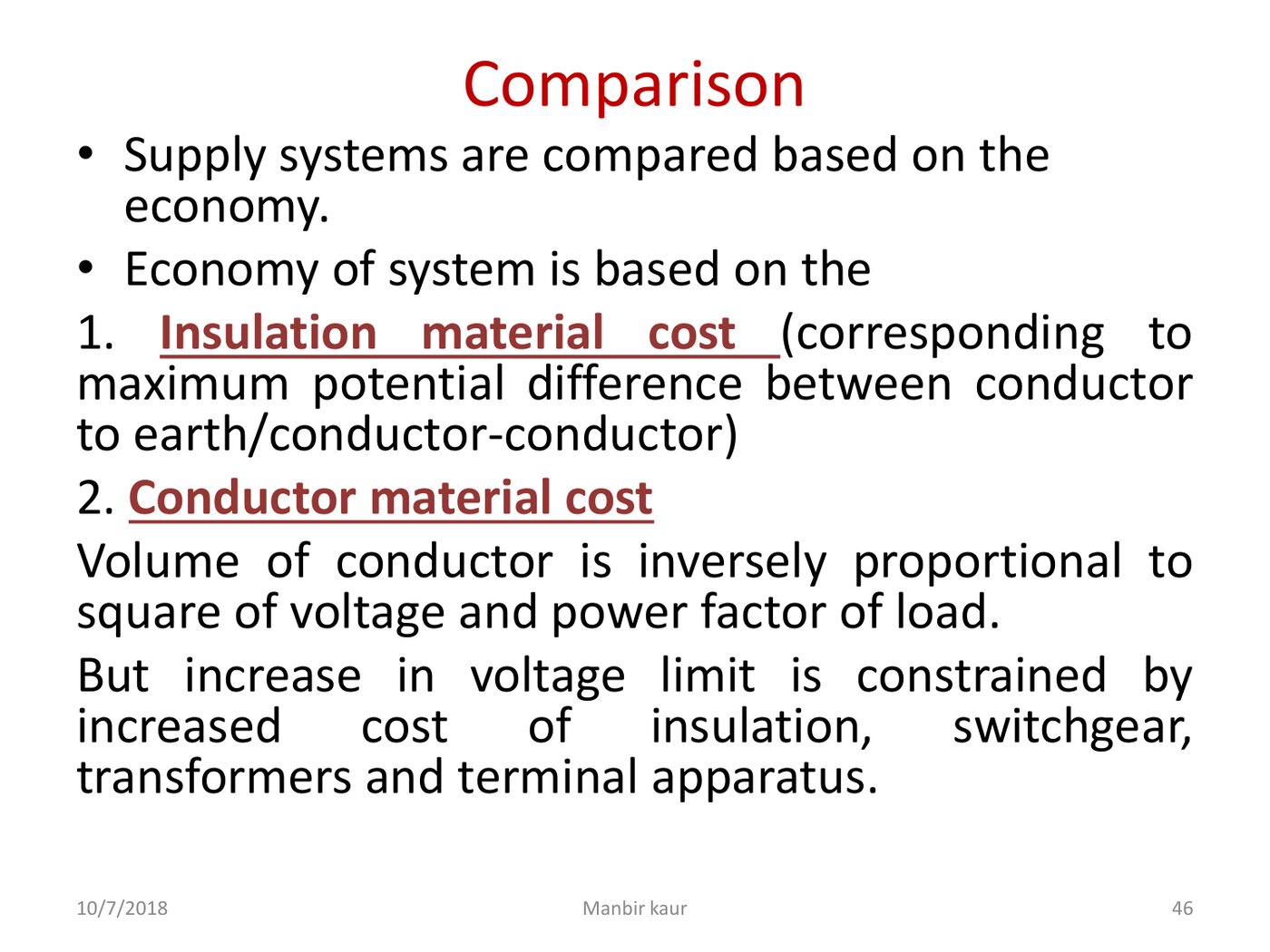
Everything in Sheet 1 is that one equation read in different directions: V² in the denominator is why we go to 220 kV and 400 kV instead of sending power at 400 V, and cos²θ in the denominator is why a bad power factor costs real copper. The limit is not electrical but economic — insulation, switchgear and transformers all get more expensive with voltage, which is the trade-off her comparison slide opens with. Unlocks Q1–Q4.

2 · Why we normalise everything (per unit)

A real system is a chain of different voltages welded together by transformers. Referring every impedance through every turns ratio by hand is arithmetic with no insight in it. So pick one power base for the whole system and one voltage base per zone, express everything as a fraction of its own base, and the turns ratios cancel identically:

Base impedance, per zone Z_base = (kV_base)²MVA_base · Z_pu = Z_ohms / Z_base

What survives is a single circuit you can solve like a first-year exercise, in which a transformer is just a series reactance and its delta/star marking is irrelevant. Two things are then non-negotiable: the voltage bases must propagate by the transformer nameplate ratio, not by whatever voltage the system happens to be running at, and a manufacturer's per-unit reactance is quoted on his rating, so it must be re-based onto yours. Unlocks Q5–Q7. Not in the decks — Wadhwa §1.5.

3 · Where inductance comes from, and why the radius shrinks

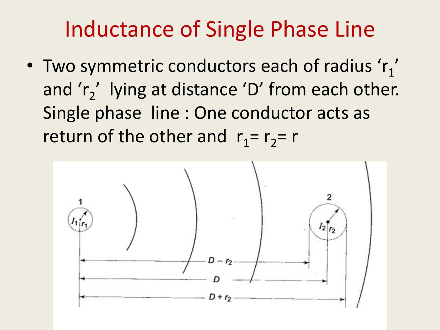
Current makes a magnetic field; the field threading a circuit is flux linkage; inductance is flux linkage per ampere. For a long straight conductor the field outside falls as 1/x, so integrating from the conductor surface out to the return path produces a logarithm — that is why every inductance answer on Sheet 4 is a log of a ratio of two distances. Flux also links current inside the conductor, and doing that integral honestly is exactly equivalent to pretending all the current flows on a slightly smaller radius:

Inductance per phase, per metre L = 2×10⁻⁷ ln D_eqD_s H/m, with r′ = 0.7788 r = e^−1/4 r

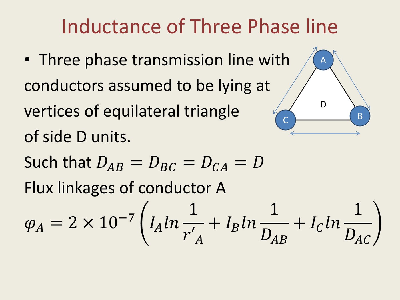
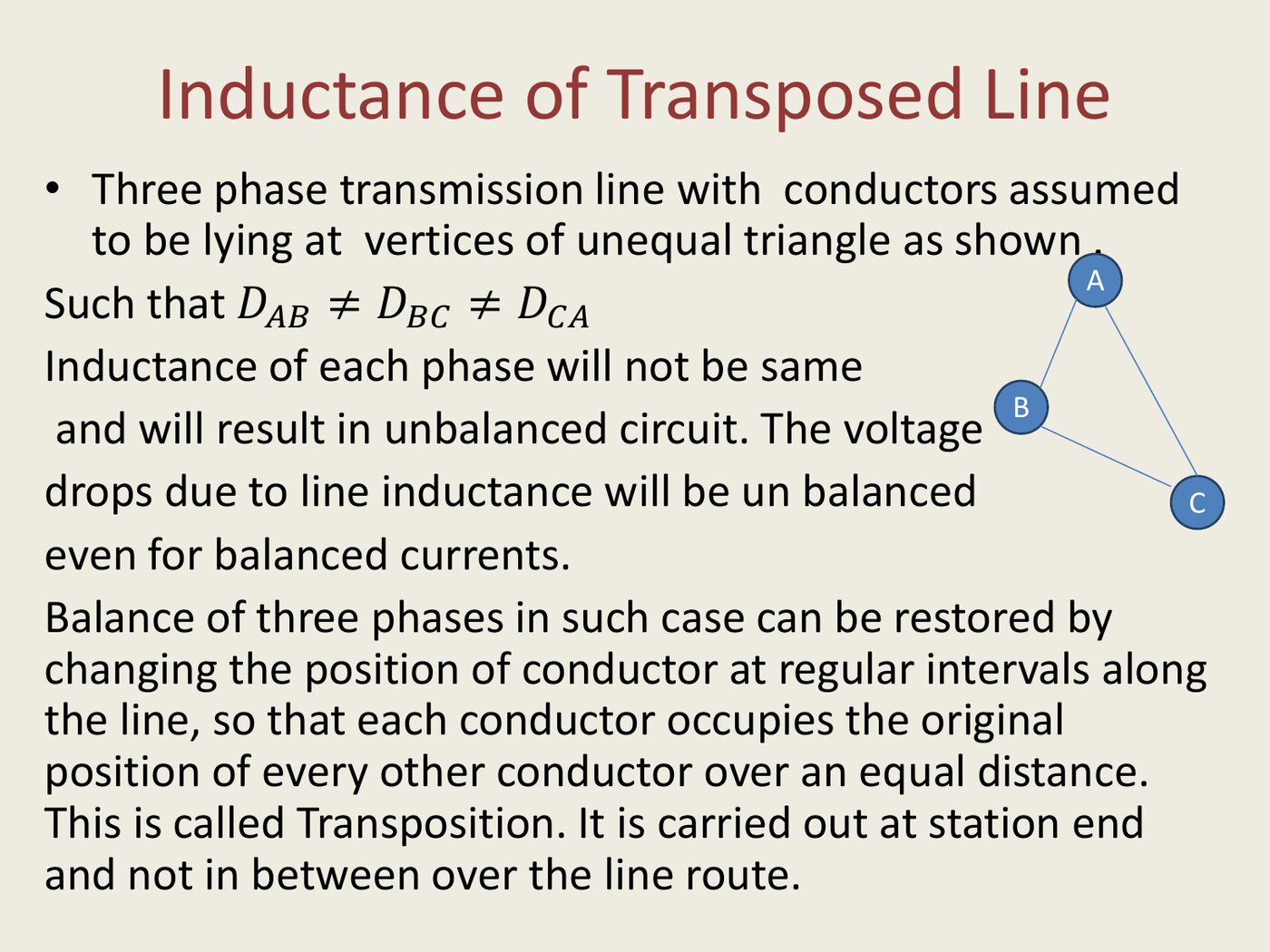
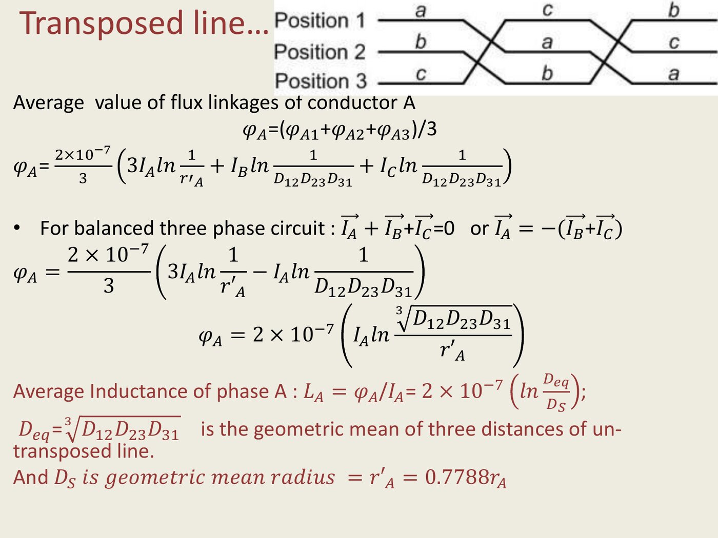
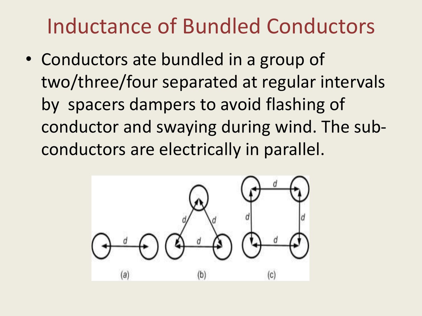
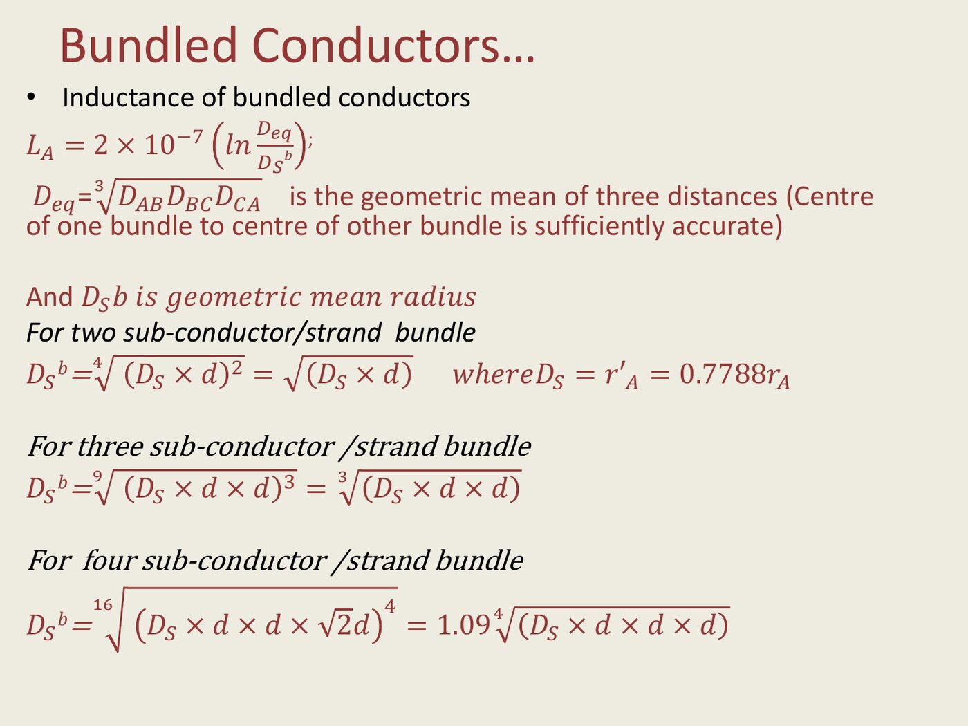
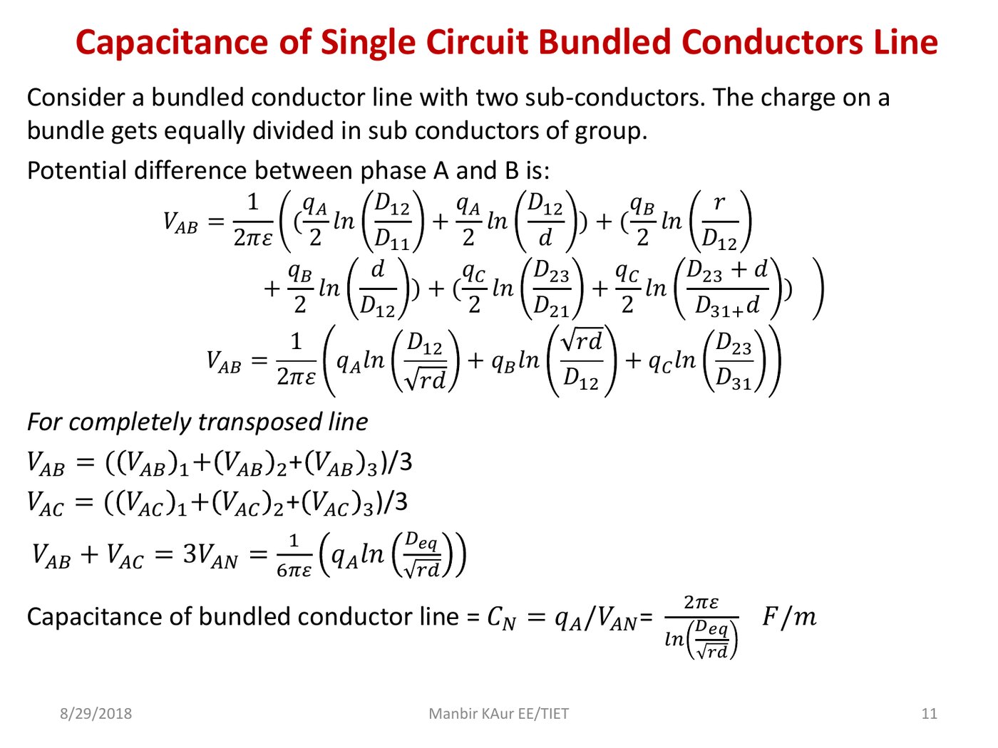
The 0.7788 is not a fudge factor — it is e^−1/4, the price of the internal flux. Two more ideas ride on the same formula. Transposition: with unequal spacing each phase links a different flux, so the three inductances differ and the line is unbalanced; rotating each conductor through all three positions over equal distances averages them, and the average is the geometric mean D_eq = ³√(D₁₂D₂₃D₃₁). Bundling: splitting a phase into subconductors makes the phase look electrically fatter, which lowers inductance and — more importantly in real EHV lines — lowers the surface field that would otherwise cause corona. Unlocks Q11–Q13, Q16.

4 · Where capacitance comes from, and why it uses a different radius

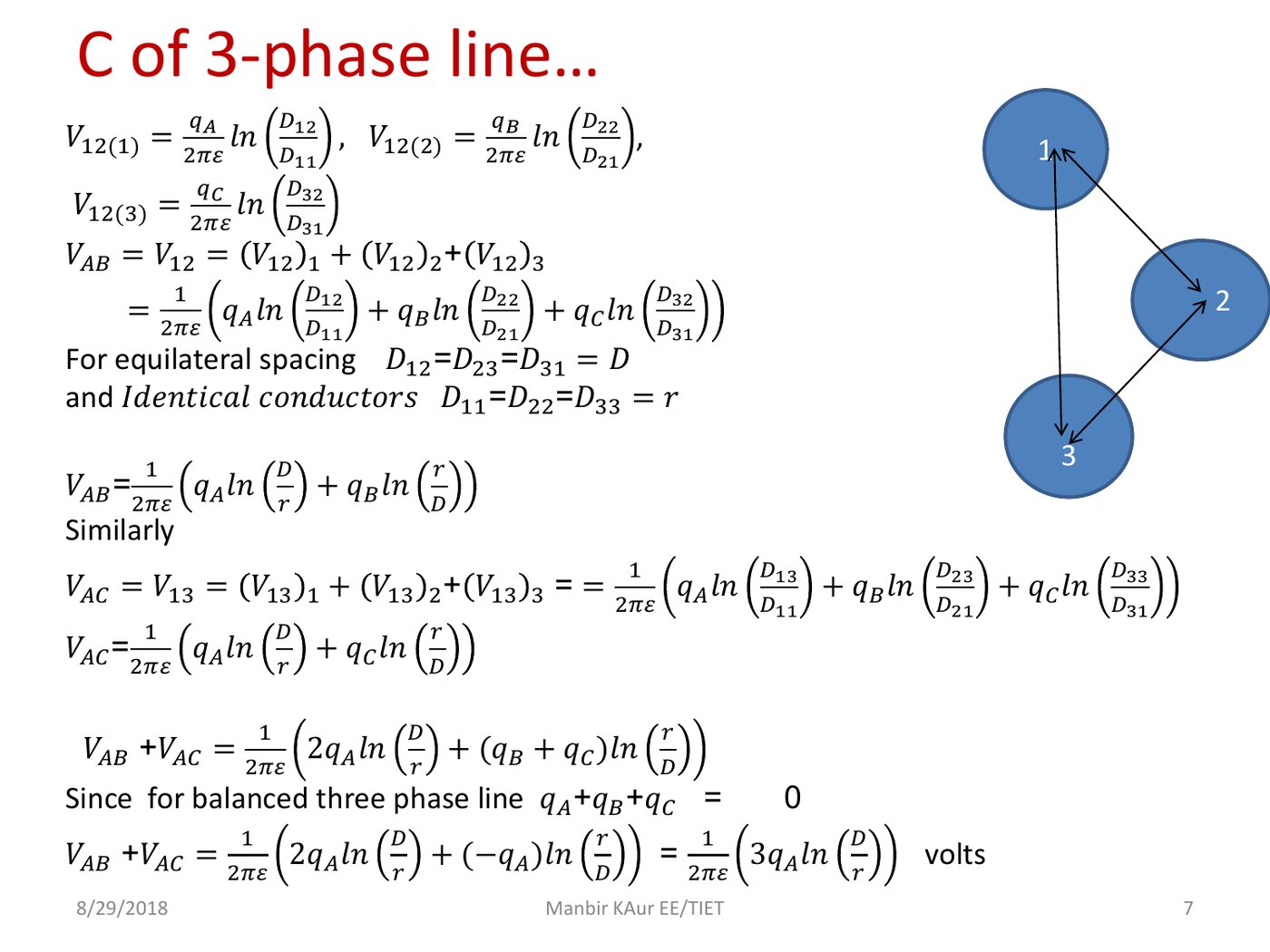
Voltage makes an electric field, and by Gauss's law the field around a charged conductor also falls as 1/x — so capacitance is again a logarithm of a ratio, with the constant ε₀ instead of µ₀:

Capacitance to neutral, per metre C = 2π ε₀ln ( D_eq / r ) F/m

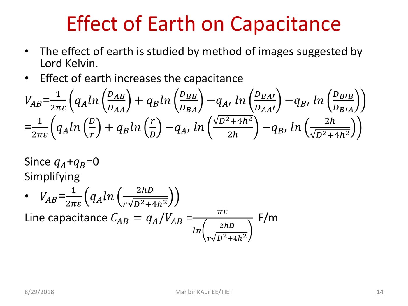
But charge sits on the surface of a conductor and there is no field inside it, so there is no internal term to absorb — the radius here is the true r, never 0.7788 r. That single asymmetry is the most common lost mark on Sheet 4. Two consequences worth holding: this capacitance draws a charging current even with no load connected, which is why a long line generates reactive power; and the earth acts as a mirror, adding an image charge of opposite sign whose attraction always increases the capacitance — by only a fraction of a percent when the conductors hang far above ground, which is why it is usually ignored. Unlocks Q14–Q17.

5 · The line as a mechanical object

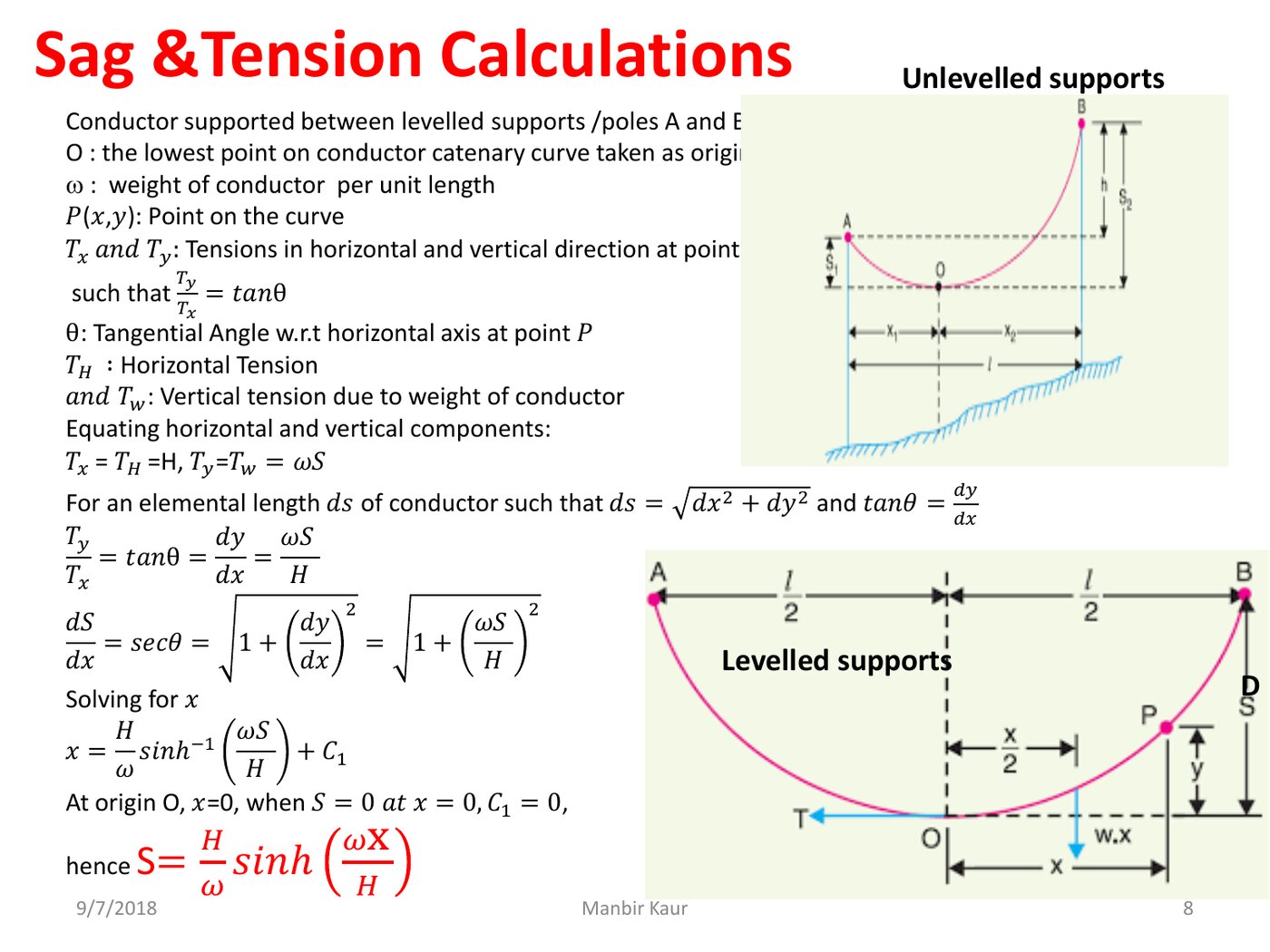
Forget electricity for two sheets. A conductor hung between two towers is a flexible cable under its own weight, so it takes the shape of a catenary. When the sag is small compared with the span — true for every span you will be asked about — the catenary is indistinguishable from a parabola, and the algebra collapses to

Sag, level supports S = w L²8 T (equivalently ωl²/2T with l = half-span)

Sag and tension trade off directly: pull it tighter and it sags less but the conductor is closer to breaking, which is why a factor of safety divides the ultimate strength. Then the weather adds load as vectors: ice coats the conductor and acts straight down, wind pushes horizontally on the projected area, and the resultant tilts the whole sag plane by an angle γ. This is why the question "which sag?" has two answers — the slant sag along the resultant, and the vertical sag, which is the one that decides whether the line clears the ground. Unlocks Q18–Q20.

6 · Insulation: the field is what fails, not the voltage

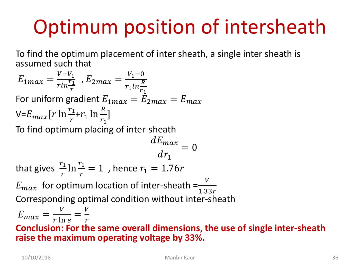
Air breaks down at about 30 kV/cm and cable dielectrics at a few tens of kV/mm. What matters is therefore never the voltage itself but the field strength it produces, and in any cylindrical geometry the field is worst right at the conductor surface:

Stress in a single-core cable E(x) = q2π ε x → E_max = Vr ln(R/r)

Two whole sheets follow from that expression. Minimising E_max over r gives ln(R/r) = 1, so R/r = e — the "most economical size" that looks like magic until you differentiate. Grading attacks the same peak from the other side: use several dielectrics, highest permittivity next to the core, so each layer runs at its own permissible stress and the wasteful margin in the outer layers disappears. And a suspension insulator string is the same problem in discrete form: the units form a capacitive divider, but each metal cap also has a stray capacitance to the earthed tower, which steals current from the units above — so the unit nearest the line conductor carries the most voltage and fails first. A guard ring feeds that stolen current back. Unlocks Q21–Q30.

The one habit that makes all six ideas usable

Notice that four of the six formulas above are a logarithm of one distance divided by another. That is not a coincidence — it is what a 1/x field integrates to. So when you meet an unfamiliar geometry, do not look for a new formula: work out what plays the role of the self distance (how big the conductor looks to its own field) and what plays the role of the mutual distance (how far away the return path is), and you already have the answer.

Sheet 1 · Q1–Q4 Unit 1

Which supply system uses the least copper

Comparing dc, single-phase, two-phase and three-phase systems that all deliver the same power over the same distance with the same losses.

Here is the whole idea. Fix the power P you must deliver, the distance l, and the power you are willing to waste as heat W. Then ask: how much conductor metal does each wiring arrangement need? The winner is whichever needs the least volume, because metal is what you buy.

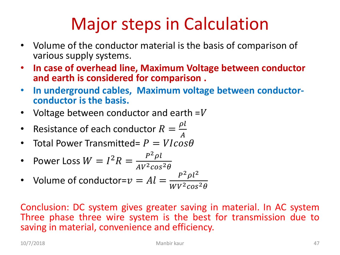
Chase the algebra through and the volume falls out. Each conductor has R = ρl/A. The current needed to deliver P at voltage V and power factor cos θ is I = P/(V cos θ). Losses are W = I²R. Eliminate I and A, and the volume v = A·l is left holding everything that matters:

Volume of conductor material v = A·l = P² ρ l²W V² cos²θ

Ppower delivered to the load (W)
ρresistivity of the conductor metal (Ω·m)
llength of the line (m)
Wtotal power lost as heat in the conductors (W)
Vvoltage — and which voltage is the whole question
cos θload power factor; dc has no power factor, so cos θ = 1

Read the two right-hand columns correctly

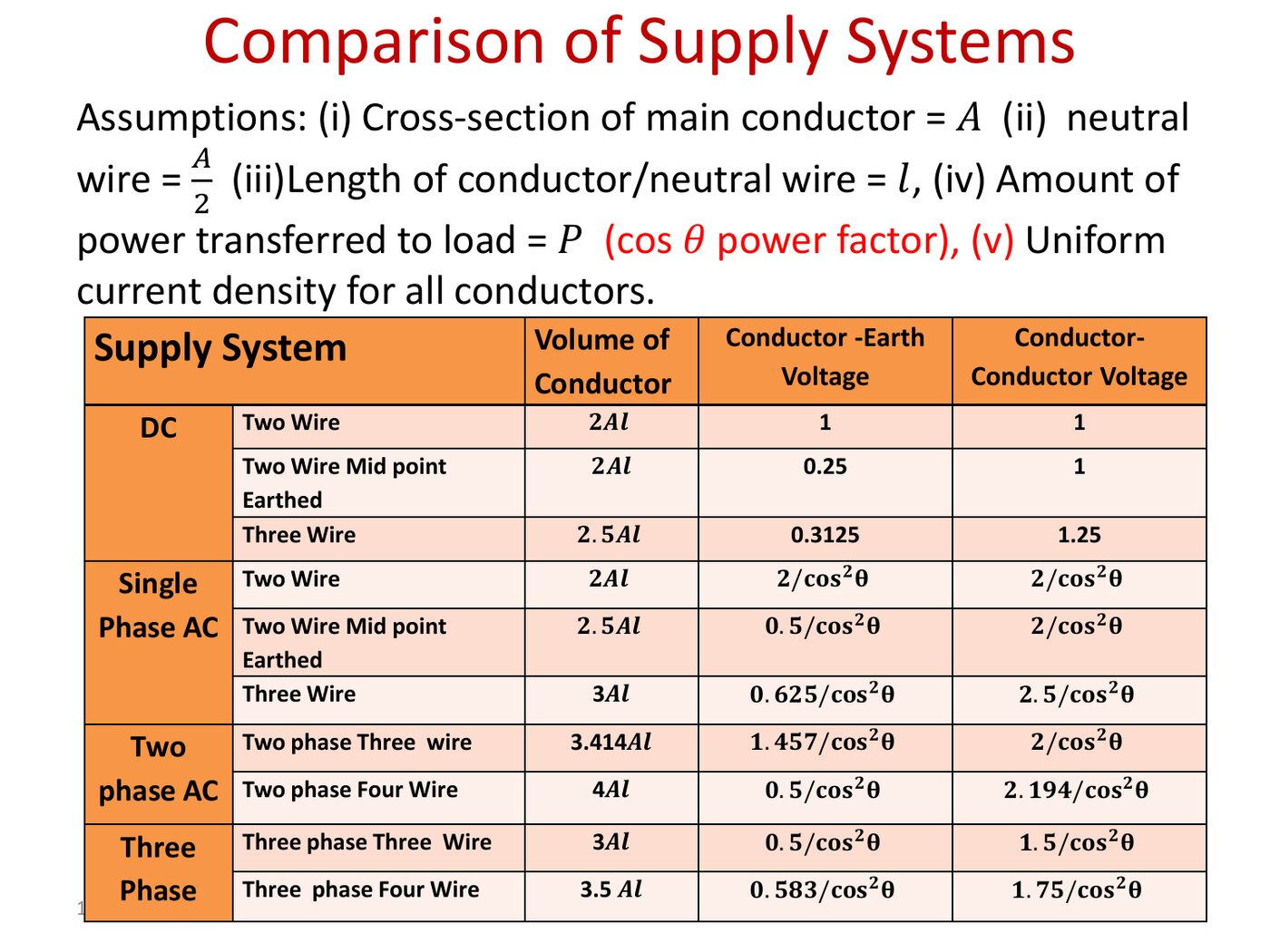
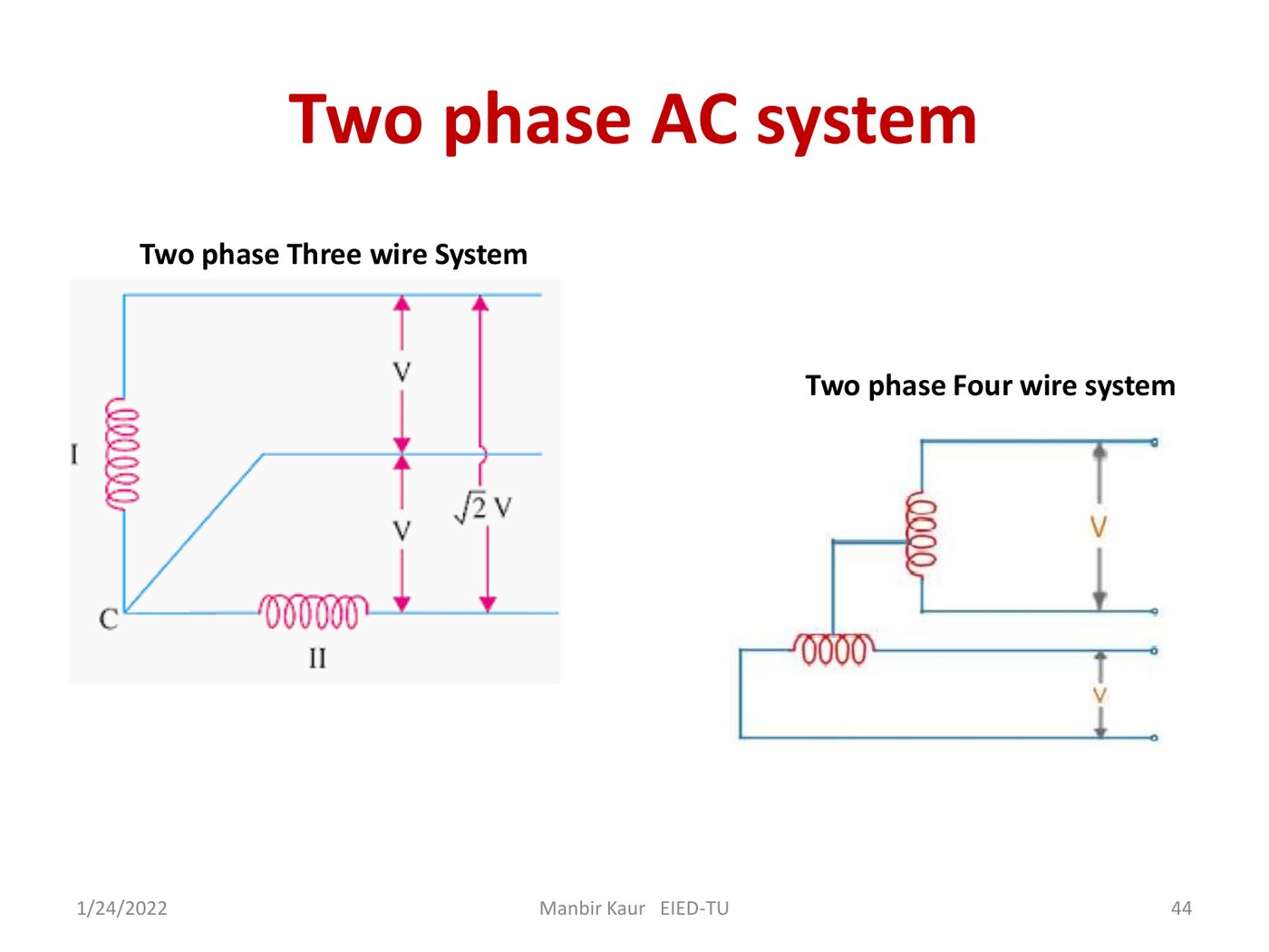
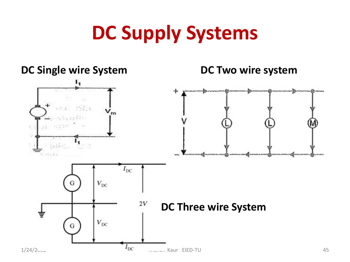
This is Unit 1's comparison table, and it is the answer to Q1 — provided you take the right column. The numbers are relative volumes, not voltages. "Conductor–earth" is the ranking when every system has the same voltage from a conductor to earth (the overhead-line constraint). "Conductor–conductor" is the ranking when every system has the same voltage between conductors (the cable constraint, and what Q1 states).

Assumptions behind every row: main conductor area A, neutral A/2, length l, power P at cos θ, uniform current density. Highlighted: the dc winner and the ac winner.
System	Configuration	Volume	Same V to earth	Same V line–line
DC	Two wire	2Al	1	1
DC	Two wire, midpoint earthed	2Al	0.25	1
DC	Three wire	2.5Al	0.3125	1.25
1-φ AC	Two wire	2Al	2 / cos²θ	2 / cos²θ
1-φ AC	Two wire, midpoint earthed	2.5Al	0.5 / cos²θ	2 / cos²θ
1-φ AC	Three wire	3Al	0.625 / cos²θ	2.5 / cos²θ
2-φ AC	Three wire	3.414Al	1.457 / cos²θ	2 / cos²θ
2-φ AC	Four wire	4Al	0.5 / cos²θ	2.194 / cos²θ
3-φ AC	Three wire	3Al	0.5 / cos²θ	1.5 / cos²θ
3-φ AC	Four wire	3.5Al	0.583 / cos²θ	1.75 / cos²θ

Q1 solved by reading the table

Q1 holds the conductor-to-conductor voltage the same across all seven systems and asks which is most economical. So: rank the last column, smallest first.

2-wire dc — 1.00

3-wire dc — 1.25

3-φ 3-wire — 1.50 / cos²θ

3-φ 4-wire — 1.75 / cos²θ

1-φ 2-wire and 2-φ 3-wire — 2.00 / cos²θ (tied)

1-φ 3-wire — 2.50 / cos²θ

So 2-wire dc is most economical overall and 3-φ 3-wire is the best ac system — which is exactly the conclusion Unit 1 states, and why the grid is three-phase three-wire everywhere it can be.

Trap · the cos²θ makes ac look worse than it is

Every ac entry carries 1/cos²θ, so at cos θ = 0.8 the 3-φ 3-wire figure is 1.5/0.64 = 2.34, worse than 3-wire dc. That is real, not an error — poor power factor genuinely costs copper. It is also why "improve the power factor" is the cheapest upgrade a utility can buy.

Trap · Q2 and Q4 are not table lookups

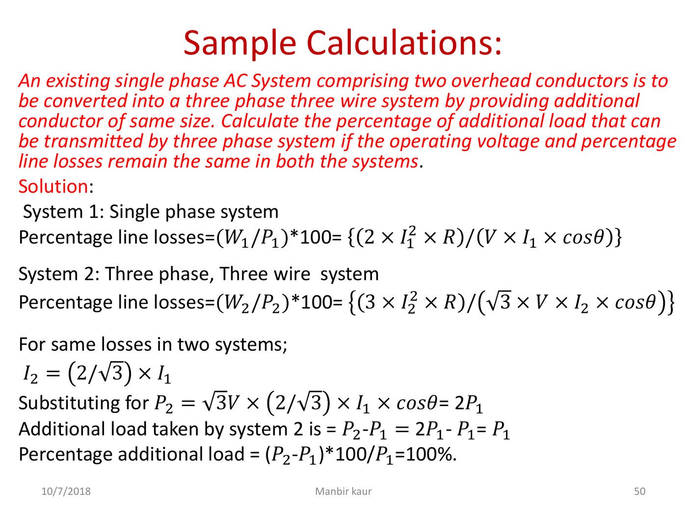
Q2 (3-wire dc → 3-φ 3-wire) and Q4 (2-wire vs 3-wire dc costing) want the algebra done from scratch under their constraint. Unit 1 has a worked twin of Q2 on slide 50 — the 1-φ → 3-φ conversion. Follow its shape: write % loss for each system, set them equal, solve for the power ratio. For Q4, carry it all the way to rupees: volume → mass via density → cost via Rs 95/kg.

Trap · Q3 is a different animal

Q3 is not economics at all — it is an unbalanced-load current calculation hiding in Sheet 1. There are two load layers: a balanced 500 kW at 0.8 pf lagging, plus three different single-phase loads (75 kW upf, 120 kW at 0.85, 150 kW upf) hung between each line and neutral. Convert each layer to a current phasor per phase (magnitude P/(V_ph·pf), angle = −cos⁻¹pf), then add the two layers per phase as vectors, not as numbers. With 400 V line-to-line, V_ph = 231 V.

Q1Rank seven supply systems Read the "same V line–line" column. 2-wire dc wins; 3-φ 3-wire is the best ac. dc 2-wire 1.00 · dc 3-wire 1.25 · 3-φ 3-wire 1.50 — computed here

Q23-wire dc → 3-φ 3-wire, extra load Equal max line voltage and equal % loss. Set %W equal for both systems, solve for the power ratio. Slide 50 of Unit 1 is the same problem with 1-φ as the starting system. P₂ = 2P₁cos²θ → +100 % at unity pf — computed here

Q3Line currents, 3-φ 4-wire, unbalanced V_ph = 400/√3 = 231 V. Balanced share + line-to-neutral load, added as phasors per phase. 1178 · 1512 · 1474 A, neutral 604 A — computed here

Q4Conductor cost, 2-wire vs 3-wire dc Equal efficiency → equal % loss. Volume → mass (6.6 g/cc) → cost (Rs 95/kg). Middle wire is half-area. 3-wire = 0.3125 × 2-wire cost (saves 68.75 %) — ratio only

Q3, drawn. Each line current is two arrows added head to tail: its share of the balanced 500 kW load, then its own line-to-neutral load. The angles are measured from that phase's own voltage, which is why the three resultants are not 120° apart. The inset shows why the neutral only sees the unbalance.

Unit 1, as she taught it

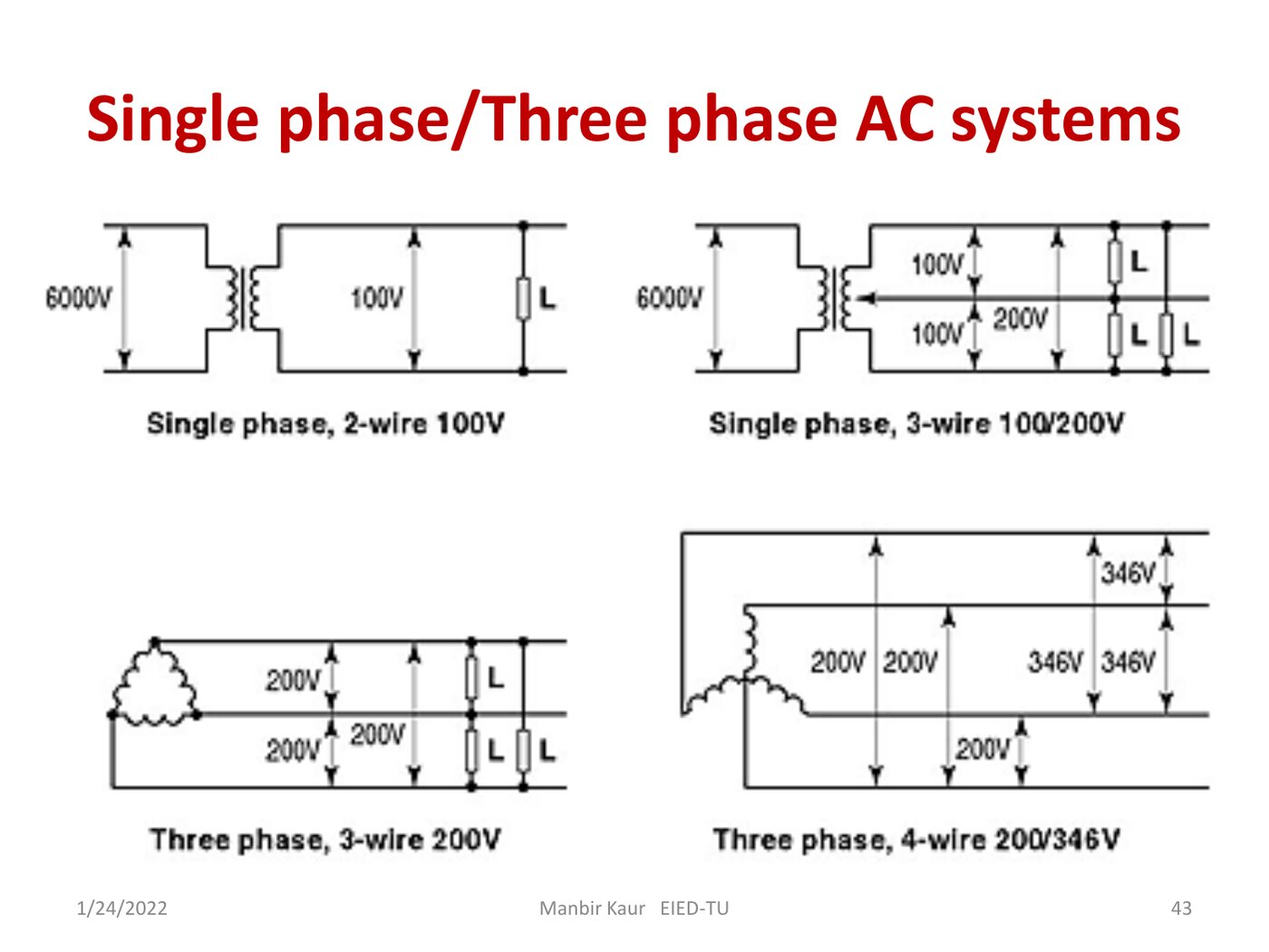
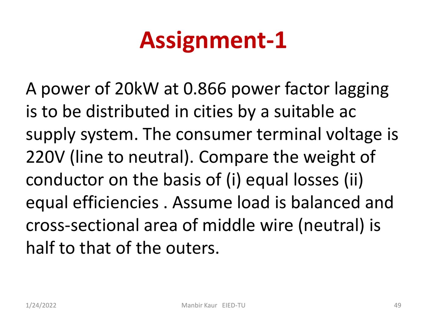
Eight slides carry everything Sheet 1 needs: the system diagrams you are being asked to rank, the volume-of-conductor derivation, the comparison table itself, and her own worked version of Q2.

Unit 1, as she taught it — slide 47 — **Where that table comes from.** v = P²ρl²/(WV²cos²θ) — volume falls with the square of both voltage and power factor. Every Sheet 1 comparison is this one line. (U1 slide 47)

Unit 1, as she taught it — slide 46 — **Why comparison is about two costs.** Insulation cost rises with voltage, conductor cost falls with it — the reason the ranking is not simply 'use more volts'. (U1 slide 46)

Unit 1, as she taught it — slide 43 — **Single-phase and three-phase configurations.** 2-wire, 3-wire mid-point-earthed, 3-φ 3-wire, 3-φ 4-wire — the rows of the table, drawn. (U1 slide 43)

Unit 1, as she taught it — slide 44 — **Two-phase systems**, three-wire and four-wire. Rarely used in practice, still in the table. (U1 slide 44)

Unit 1, as she taught it — slide 45 — **DC systems**: single-wire (earth return), two-wire, three-wire. The 2-wire dc case is the reference every other row is divided by. (U1 slide 45)

Unit 1, as she taught it — slide 50 — **Q2, already worked for you** — with single-phase as the starting system instead of 3-wire dc. Same algebra, same landing point: 100 % additional load. (U1 slide 50)

Unit 1, as she taught it — slide 49 — **Assignment-1, and the sentence that settles Q4.** 'Consumer terminal voltage is 220V (line to neutral)' — read it as outer-to-outer instead and Q4's answer inverts. (U1 slide 49)

Sheet 2 · Q5–Q7 Not in the unit decks — Wadhwa §1.5, pdf p26

Per unit: making transformers disappear

Rewriting every impedance as a fraction of a chosen base, so that turns ratios stop mattering and the whole network becomes one simple circuit.

A real power system is a chain of transformers at different voltages. Referring impedances back and forth through each turns ratio by hand is miserable and error-prone. The per-unit system removes the problem: pick one power base for the whole system and a voltage base for each voltage level, express everything as a fraction of its base, and every transformer's turns ratio quietly cancels. The multi-voltage network becomes a single circuit you can solve like a first-year exercise.

Two formulas do all the work. The first converts an ohm value into per unit. The second — the one both Q5 and Q6 are really testing — moves a per-unit value that a manufacturer quoted on the machine's own rating onto your chosen system base.

Ohms → per unit Z_pu = Z_Ω · MVA_base(kV_base)²

Base impedance, if you prefer two steps Z_base = (kV_base)²MVA_base Ω

Changing base — the one that matters Z_new = Z_old · MVA_newMVA_old · (kV_old)²(kV_new)²

oldthe nameplate rating the % reactance was quoted on
newthe system base you were told to use

Q5, first machine, start to finish

Generator: 10 MVA, 13.2 kV, 16% reactance. New base: 50 MVA, 13.8 kV.

16% → 0.16 pu on its own base (percent ÷ 100, always first)

X = 0.16 × (50/10) × (13.2/13.8)²

= 0.16 × 5 × 0.9147

= 0.7318 pu

Then repeat, mechanically, for the other three machines: generator 2 uses 50/15, and both motors use their own MVA with (12.5/13.8)² = 0.8203. G1 0.732 · G2 0.488 · M1 1.077 · M2 0.718 pu

Trap · a bigger base gives a bigger per-unit reactance

Notice the MVA ratio sits on top. Moving a 10 MVA machine onto a 50 MVA base multiplies its per-unit reactance by five. If your number got smaller when the base MVA got bigger, you inverted a ratio. Sanity-check every conversion against that sentence.

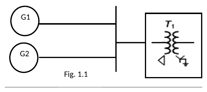
Trap · Q6's delta–star transformer is a decoy

The transformer is 11 kV delta / 66 kV star, which invites you to start juggling √3. Don't. In per unit, a transformer is one series reactance; the winding connection does not enter. Put both generators in parallel (they are on the same bus), add the transformer reactance in series, then convert the total back to ohms at the 66 kV side with Z_base = 66²/35 = 124.5 Ω. That "back to ohms" step is what the question is asking for.

Trap · Q7 wants the same circuit three ways

Part (a) is deliberately the tedious version — refer impedances through turns ratios by hand, both directions, in ohms. Part (b) is the same system in per unit. Part (c) then asks for the sending-end voltage. Do part (a) honestly; the contrast with (b) is the entire lesson of the sheet. Watch the transformer nameplates: A–B is 500 V/1.5 kV but the base for circuit B is 1.2 kV, so the voltage bases on the two sides of that transformer are not its nameplate ratio.

Fig. 1.1 — generators G1 and G2 on a common bus feeding transformer T1, 11 kV delta / 66 kV star — **Fig. 1.1, as printed on Sheet 2.** Q6's system: G1 and G2 both land on the same bus, and that bus feeds the single transformer T1 (11 kV delta / 66 kV star). Two machines on one bus means *parallel*; the delta–star marking changes nothing in per unit.

Q5Four machines onto a common base Base-change formula, four times. Percent → pu first. G1 0.732 · G2 0.488 · M1 1.077 · M2 0.718 pu

Q6Through impedance in ohms Generators in parallel + transformer in series, all on 35 MVA / 66 kV, then × Z_base = 124.5 Ω to get back to ohms. j18.24 Ω per phase at 66 kV (0.1466 pu) — computed here

Q7Two transformers, a line, and a load (a) ohms by turns ratio, (b) per unit on 10 kVA / 1.2 kV, (c) sending-end voltage. V_send = 1.0611 pu ∠4.03° = 424.4 V — computed here

Q7's three base zones. The callout is the whole question: circuit A bases at 400 V, not the transformer's 500 V nameplate, because circuit B is pinned at 1.2 kV. Get that wrong and every per-unit value downstream is wrong by a consistent-looking factor.

Sheet 3 · Q8–Q9 In neither the decks nor Wadhwa

What losses cost, and Kelvin's law

Costing a year of I²R heating, then choosing the conductor size where copper stops paying for itself.

Two questions, two halves of one argument. First: a load cycle wastes energy as heat all year — what is the bill? Second: a fatter conductor wastes less, but costs more to buy — where is the optimum? The second is Kelvin's law, and the reasoning is short enough to reconstruct from memory in an exam, which is just as well, since it is in none of your material.

Part one: costing a load cycle

Losses go as current squared, so you cannot average the load and then square it — you must square each block of the cycle and then add. This is the single most common mistake on Q8.

Per block of the load cycle I = P√3 · V_L · cos θ loss = 3 I² R

Then, over the cycle energy = Σ (loss_k × hours_k) → × 365 → × rate

Q8 worked through, all three blocks

11 kV three-phase line, R = 0.19 Ω. Cycle: 2.4 MW at unity for 6 h, 0.8 MW at 0.8 lag for 6 h, 0.4 MW at unity for 12 h. Energy at Re 1.00 per unit.

I₁ = 2.4×10⁶ / (√3 · 11000 · 1.0) = 126.0 A → 3I²R = 9.049 kW

I₂ = 0.8×10⁶ / (√3 · 11000 · 0.8) = 52.49 A → 3I²R = 1.570 kW

I₃ = 0.4×10⁶ / (√3 · 11000 · 1.0) = 21.00 A → 3I²R = 0.251 kW

daily = 9.049(6) + 1.570(6) + 0.251(12) = 66.73 kWh

annual = 66.73 × 365 = 24 357 kWh → Rs 24 357

The sheet prints Rs 24 359 — a two-rupee rounding gap. If you land within a few rupees, you are right.

Part two: Kelvin's law, derived in four lines

Split the annual cost of a line into the part that grows with conductor area a and the part that shrinks with it.

Annual capital charge. The line costs (fixed + variable·a) to build, and you pay interest and depreciation on it each year. Only the variable part depends on a, so only that part enters the optimisation — the fixed rupees are there whatever you choose.
Annual loss cost. Resistance goes as 1/a, so loss energy and its cost go as 1/a too.
Add and minimise. One term rises linearly, the other falls as 1/a. Differentiate, set to zero.
Out drops the law: at the optimum, the annual variable capital charge exactly equals the annual cost of the losses. That sentence is Kelvin's law — you can quote it and skip the calculus.

Kelvin's law (interest+dep. rate) × (variable capital cost) = (annual loss energy) × (energy rate)

Q8b · most economic cross-section

110 kV, 0.8 pf. Cost Rs (12000 + 8000a)/km, R = 0.19/a Ω/km, energy 8 paise, 10% interest and depreciation, 1 km.

I: 157.5 / 52.49 / 26.24 A (24, 8, 4 MW at 0.8)

ΣI²t = 173 629 A²h per day

annual loss = 3(0.19/a)(173629)(365)/1000

= 36 123 / a kWh

loss cost = 0.08 × 36123/a = 2889.9/a

capital = 0.10 × 8000a = 800a

— set equal (Kelvin) —

800a = 2889.9/a → a² = 3.612

a = 1.90 cm² — matches the sheet exactly.

Q9 · most economical current density

Cost Rs (2800a + 1300)/km, loss load factor 65%, 10%, energy 5 paise/kWh, ρ = 1.78×10⁻⁸ Ω·m.

R = ρ/a per km = 0.178/a Ω (a in cm²)

hours = 8760 × 0.65 loss load factor

loss = I²(0.178/a)(5694)/1000 kWh

cost = 0.05 × 1.0135 I²/a

capital = 0.10 × 2800a = 280a

— set equal (Kelvin) —

280a = 0.050677 I²/a

I²/a² = 5525 → I/a = 74.3

74 A/cm² — matches the sheet.

Trap · the fixed cost never enters

Rs 12000 in Q8b and Rs 1300 in Q9 are pure distractors. They change the total bill, not the optimum, because they do not vary with a. Including them gives an equation that will not solve cleanly — which is a useful signal you have gone wrong.

Trap · "loss load factor" is not "load factor"

Q9 gives 65% as the load factor of the losses. It is already the factor that converts peak loss into average loss, so multiply 8760 hours by it directly. Do not square it, and do not go looking for a separate load factor.

Trap · keep ρ and a in matching units

With ρ in Ω·m and a in cm², one km of conductor gives R = 1.78×10⁻⁸ × 1000 / (a × 10⁻⁴) = 0.178/a Ω. Getting this factor wrong moves the answer by a hundred, which is exactly how a plausible-looking wrong current density appears.

Q8Annual energy lost, 11 kV Square each block separately, weight by hours, ×365. Rs 24 359 — reproduced to Rs 24 357

Q8bMost economic cross-section Kelvin: 800a = 2889.9/a. 1.90 cm² — reproduced exactly

Q9Most economical current density Kelvin with loss load factor 0.65 → I/a. 74 A/cm² — reproduced as 74.3

Kelvin's law, computed from Q9's own cost data. The filled dot is the minimum of the total-cost curve; the open circle is where the rising capital charge crosses the falling cost of losses. They sit at the same area — that coincidence is the law, and it is why the fixed Rs 1300 never enters. The optimum works out at 74.3 A/cm², the sheet's 74.

Sheet 4 · Q10–Q17 Units 2 & 4

The three parameters, from geometry alone

Eight problems, one skeleton: resistance from the metal, inductance and capacitance from two distances — a self distance and a mutual distance.

This is the technical heart of the course, and it is far more repetitive than it first looks. Every inductance and capacitance answer is a logarithm of one distance divided by another:

ln ( how far apart the phases are ÷ how big the conductor effectively is )

The numerator is the mutual distance — the geometric mean of the spacings between phases, written D_eq. The denominator is the self distance — how large the conductor looks to its own field, written D_s. Learn to compute those two numbers and eight problems collapse into arithmetic.

One asymmetry you must respect: for inductance the self distance uses the reduced radius r′ = 0.7788 r, because flux also links the current inside the conductor. For capacitance it uses the true radius r, since charge sits on the surface and there is no field inside. Mixing these up is the most common error on this sheet.

Inductance per phase, per metre L = 2×10⁻⁷ · ln D_eqD_s H/m

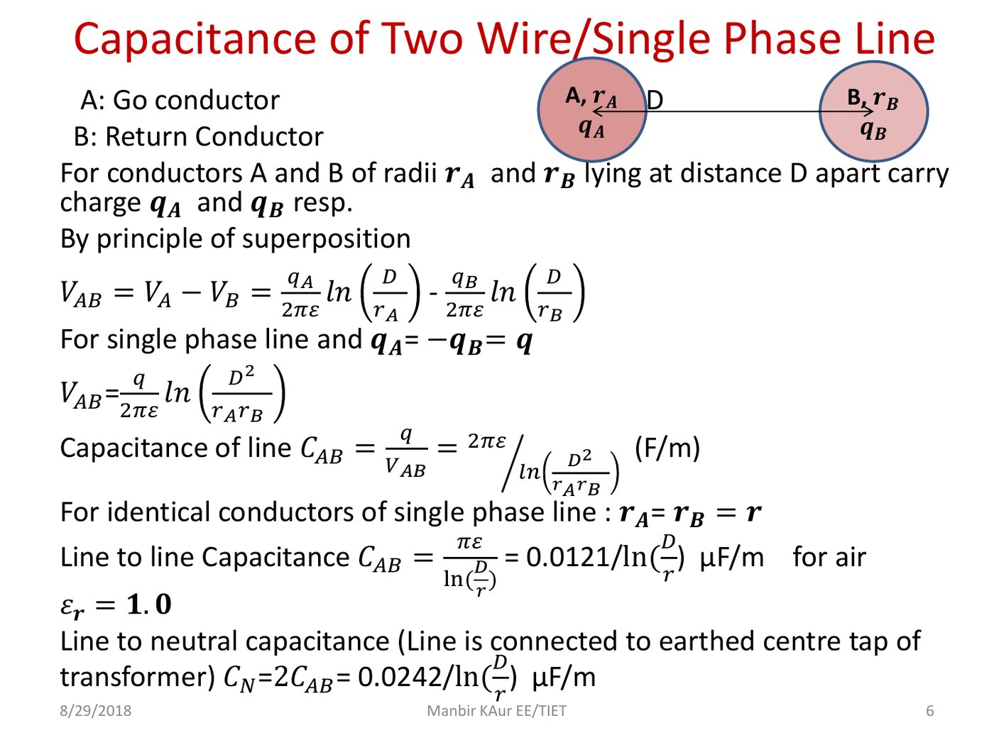
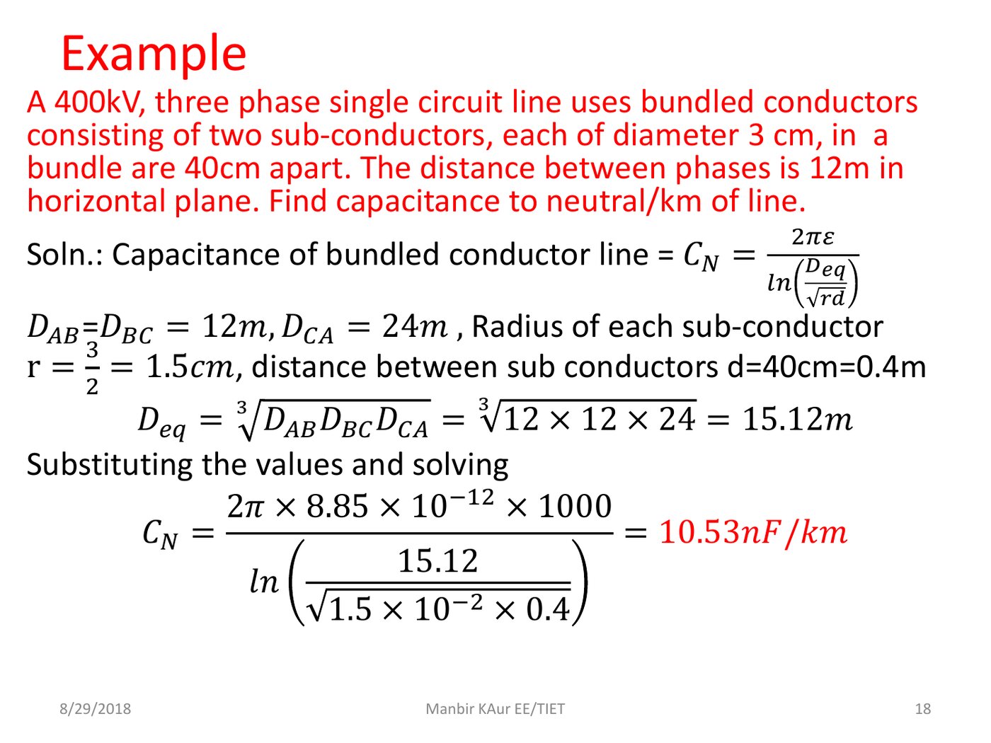
Capacitance per phase, per metre C = 2π ε₀ln ( D_eq / r ) F/m

ε₀8.854×10⁻¹² F/m
2πε₀5.5626×10⁻¹¹ — worth memorising
πε₀2.7813×10⁻¹¹ — the single-phase version

Mutual distance — unequal spacing, transposed D_eq = ³√ D₁₂ D₂₃ D₃₁

Self distance — plain conductor D_s = r′ = 0.7788 r (for L)

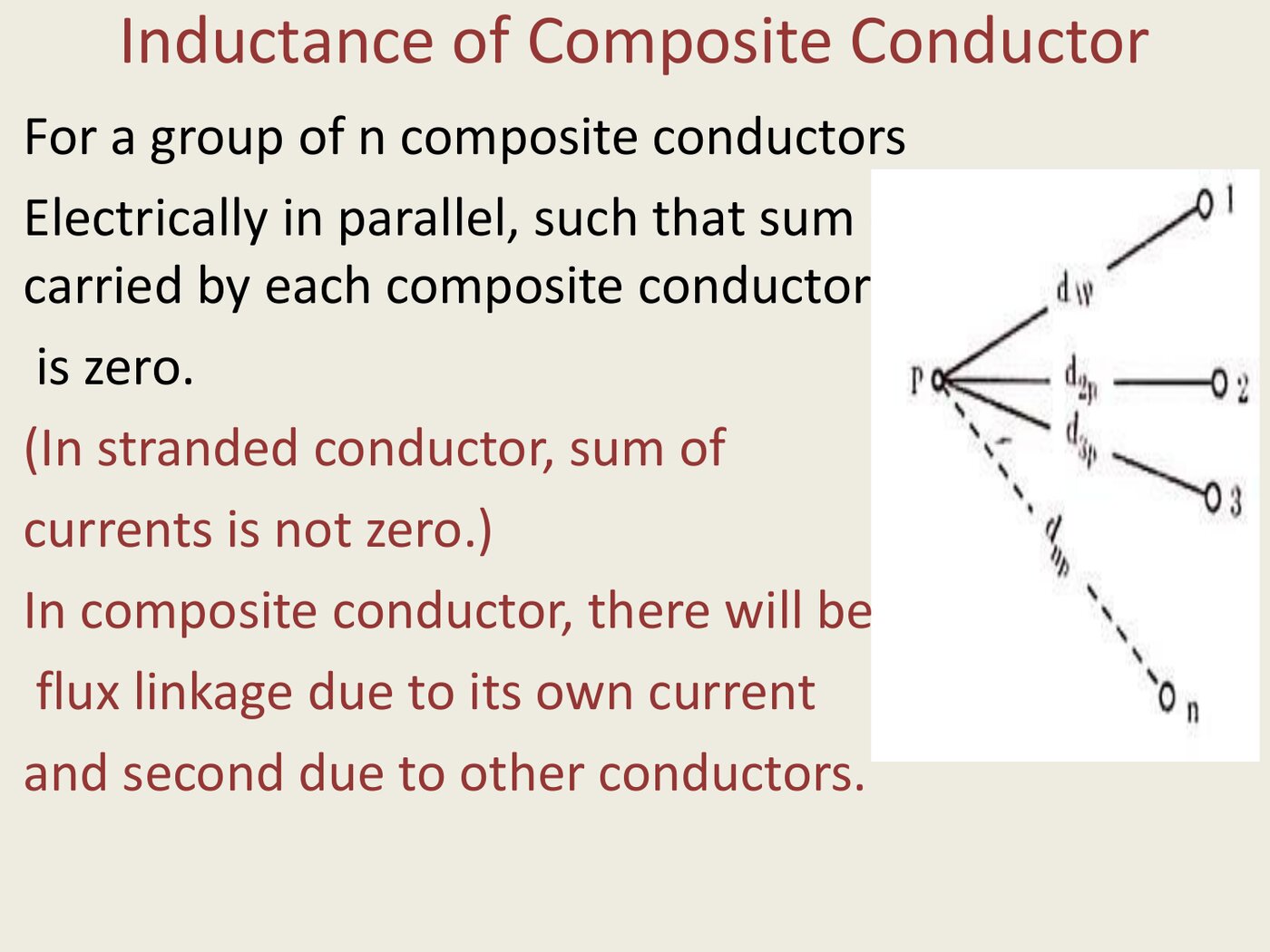
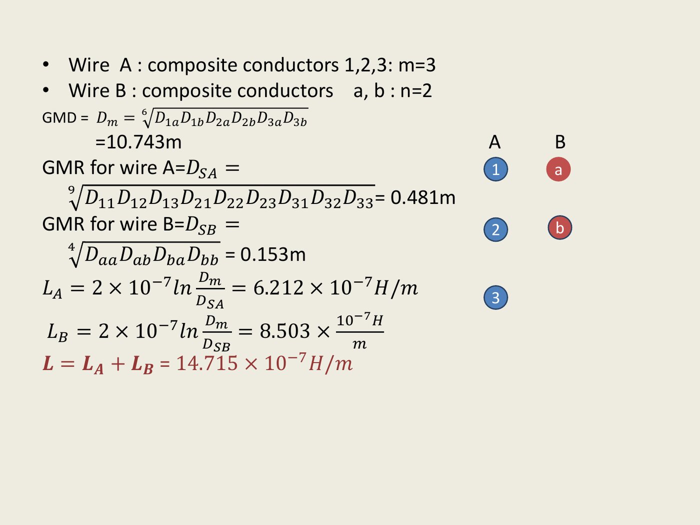
Self distance — two-conductor bundle, spacing d D_s^b = √ r′ · d (for L) r_b = √ r · d (for C)

Single-phase lines: everything doubles

A single-phase line is a loop — go and return — so its inductance is twice a single conductor's, while its capacitance is measured between two conductors and is therefore half the line-to-neutral value. Hence the 4 and the π.

L_loop = 4×10⁻⁷ · ln Dr′ H/m C_AB = π ε₀ln ( D / r ) F/m

Q11 · inductance, unequal spacing

d = 2.0 cm, spacings 4 m, 4 m, 8 m, transposed.

r = 1 cm → r′ = 0.7788 cm = 0.007788 m

D_eq = ³√(4·4·8) = ³√128 = 5.040 m

L = 2×10⁻⁷ ln(5.040 / 0.007788)

= 2×10⁻⁷ × ln 647.1

= 2×10⁻⁷ × 6.4725

= 1.2945×10⁻⁶ H/m

1.2945 mH/km per phase
The sheet prints "1.2947 H/km" — the number is right, the unit is a typo. It is mH/km. For the un-transposed part, compute each phase separately; they differ, which is why lines are transposed.

Q12 · bundled conductors (Fig. 2)

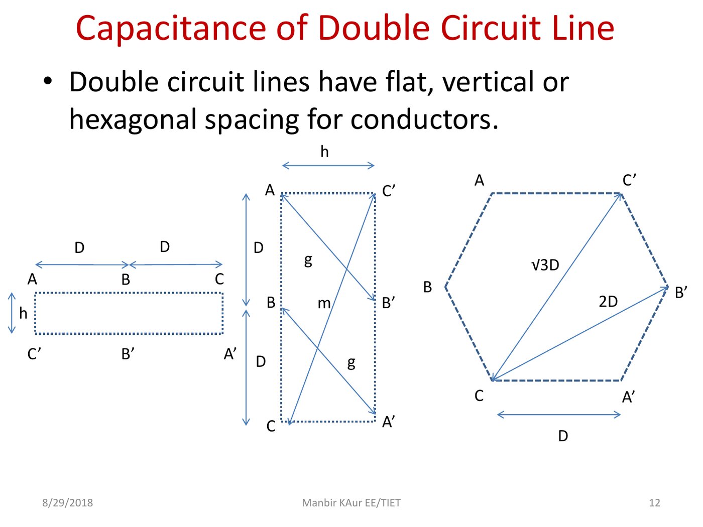
Fig. 2 is a flat 3-φ line, two conductors per phase, bundle spacing 40 cm, phase centres 6.5 m apart. Each conductor 5 cm diameter.

Fig. 2 — flat three-phase line, two-conductor bundles, 40 cm bundle spacing, 6.5 m between phase centres — **Fig. 2, as printed on Sheet 4.** Q12 and Q16 both refer to it. The docx stores it as an EMF drawing that no text extractor reads — this is the sheet re-rendered, so the geometry is the instructor's, not a reconstruction. Bundle spacing d = 40 cm, phase centres 6.5 m, so a–c is 13 m.

r = 2.5 cm → r′ = 1.947 cm = 0.01947 m

D_s^b = √(0.01947 × 0.4) = 0.08825 m

D_eq = ³√(6.5 · 6.5 · 13) = 8.189 m

L = 2×10⁻⁷ ln(8.189 / 0.08825)

= 2×10⁻⁷ × ln 92.80 = 9.061×10⁻⁷

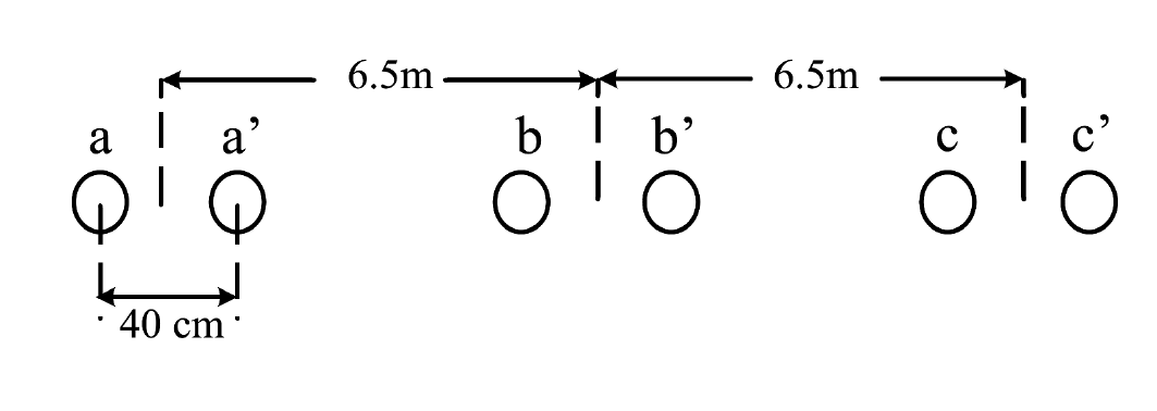
0.906 mH/km per phase — matches the sheet.

Q15 · capacitance, charging current, kVAr

3-φ, 50 Hz, d = 21 mm, spacings 3 / 5 / 3.6 m, operating at 132 kV.

r = 10.5 mm = 0.0105 m

D_eq = ³√(3 · 5 · 3.6) = 3.780 m

C = 5.5626×10⁻¹¹ / ln(360)

= 9.45×10⁻¹² F/m = 0.00945 µF/km

X_C = 1/(2πfC) ≈ 0.337 MΩ·km

V_ph = 132/√3 = 76.21 kV

I = 2πf C V_ph = 0.2263 A/km

Q = 3 V_ph I = 51.74 kVAr/km

0.226 A/km · 51.7 kVAr/km — both match.

Q17 · does the earth matter?

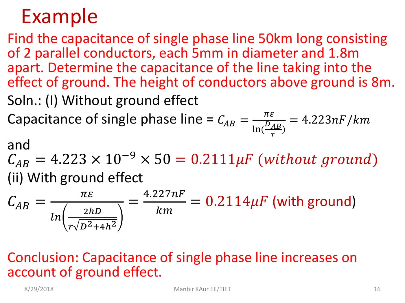
1-φ, 50 km, d = 5 mm, D = 1.8 m, conductors 8 m above ground. Compute C with and without the ground.

no ground: C = πε₀/ln(1.8/0.0025)

= 2.7813×10⁻¹¹ / 6.5793

→ 0.2114 µF over 50 km

— now add the image conductors —

correction = ln( √(D²+4h²) / 2h )

= ln(16.101/16) = 0.0063

C = πε₀/(6.5793 − 0.0063)

→ 0.2116 µF over 50 km

≈ 0.211 µF either way
A 0.1% change. That is the answer: earth always increases capacitance, but negligibly once the conductors are high compared with their spacing. Say so explicitly — it is the point of the question.

Trap · r′ for inductance, r for capacitance

0.7788 belongs to inductance only. Using it in a capacitance formula (or forgetting it in an inductance one) shifts the logarithm by 0.25 and quietly changes the answer by a few percent — small enough to look plausible, large enough to be wrong.

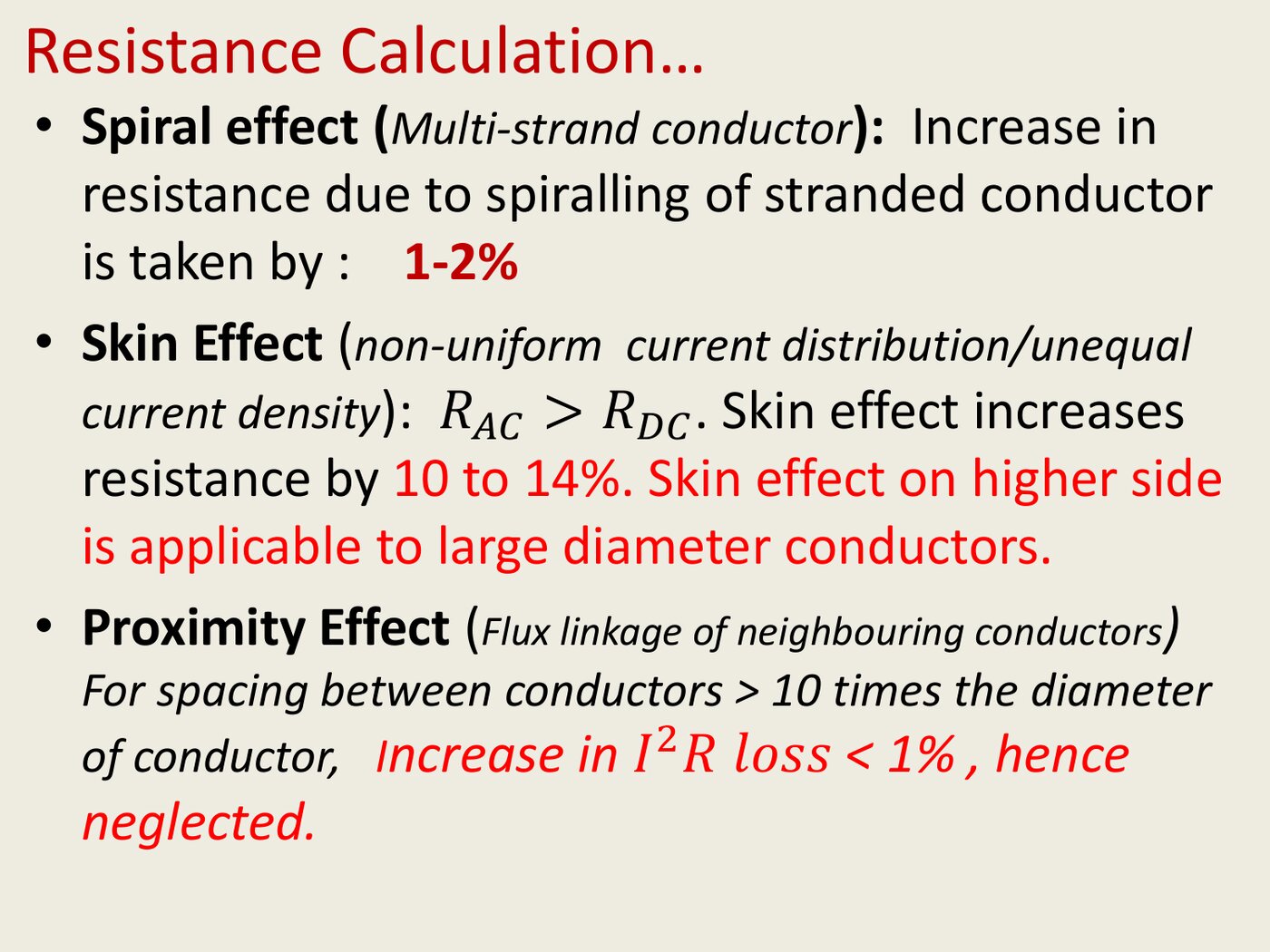
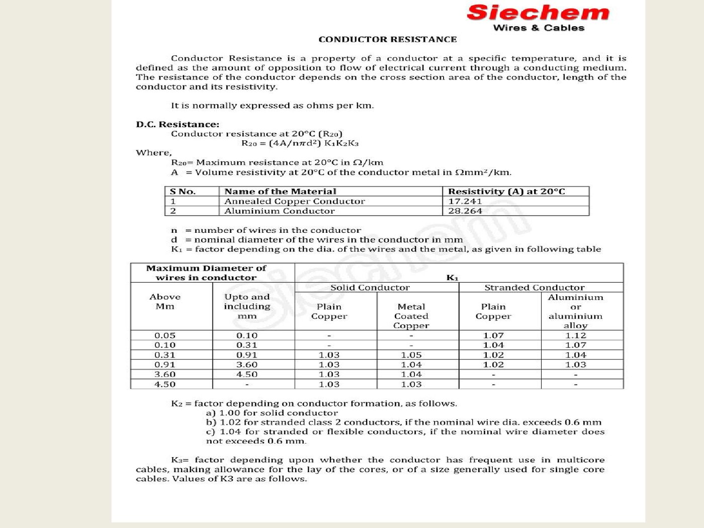
Trap · Q10's "ac resistance" is not skin effect

Total area first: 37 strands × π(0.333/2)² = 3.222 cm². Correct ρ from 20 °C to 75 °C with ρ₇₅ = ρ₂₀[1 + α(55)]. The stated 2% is for spiralling — the strands are longer than the cable because they wind helically — not for skin effect, which is negligible for this size at 50 Hz. State that assumption in your answer; the question is ambiguous about whether the 2% applies to the dc value too, so say which you did.

Trap · Q13 runs the formula backwards

You are given the reactance limit (31.4 Ω over 50 km) and must find the spacing. Work back: L = X/2πf, divide by length to get H/m, divide by 4×10⁻⁷ to get the logarithm, exponentiate, multiply by r′. Around 1.5 m. It is the same formula, just solved for the other unknown.

Trap · un-transposed means per-phase, not averaged

For an un-transposed line each phase has a different inductance, and phase B (the middle one) is the odd one out. Q11 asks for both cases so you can see the difference; do not average the three and call it done.

Q10AAC dc and ac resistance at 75 °C 37 strands → area 3.222 cm², temperature-correct ρ, add 2% for spiralling. R_dc = 0.1093 Ω/km · R_ac = 0.120–0.125 Ω/km — computed here

Q11Inductance, 4/4/8 m spacing D_eq = ³√128 = 5.04 m; r′ = 0.7788 cm. 1.2945 mH/km — sheet's "H/km" is a unit typo

Q12Bundled 460 kV line D_s^b = √(r′d) = 0.0883 m; D_eq = 8.19 m. 0.906 mH/km — reproduced exactly

Q13Maximum permissible spacing Reactance limit → L → invert the log, using the loop form 4×10⁻⁷ ln(D/r′). D = 1.48 m — computed here, plug-back gives 31.400 Ω

Q14Capacitance, 1-φ, 40 km C = πε₀/ln(D/r), then × 40 000 m. 0.1737 µF — reproduced as 0.1739

Q15C, X_C, charging current, kVAr D_eq = 3.78 m; V_ph = 76.21 kV. 0.226 A/km · 51.7 kVAr — both reproduced

Q16C and charging current, Fig. 2, 220 kV Same geometry as Q12 but capacitance: r_b = √(r·d) = √(0.025×0.4) = 0.1 m exactly. Gives ≈ 0.0126 µF/km and ≈ 0.50 A/km. 12.62 nF/km · 0.504 A/km · 192 kVAr/km — computed here

Q17Capacitance with earth effect Subtract ln(√(D²+4h²)/2h) from the denominator. Changes the answer by 0.1%. 0.2113 → 0.2115 µF — matches her Unit 4 p16, where this exact question is worked

Units 2 and 4, as she taught them

Seventeen slides: resistance corrections, then every inductance and capacitance geometry the sheet uses — including the two slides that work Q17 and check your Q16 setup.

Units 2 and 4, as she taught them — slide 12 — **The K₁ table** behind that 2 %: 1.02 for stranded class-2 conductors above 0.6 mm wire diameter, 1.04 below. Q10's '2 % due to spiralling' is this factor. (U2 slide 12)

Units 2 and 4, as she taught them — slide 18 — **Single-phase two-wire line.** Both conductors carry the same current in opposite directions, so the loop inductance is twice the per-conductor value — the trap in Q11 and Q13. (U2 slide 18)

Units 2 and 4, as she taught them — slide 21 — **Three-phase, equilateral spacing.** D_AB = D_BC = D_CA = D, so every phase sees the same inductance and no transposition is needed. (U2 slide 21)

Units 2 and 4, as she taught them — slide 25 — **Composite conductors.** GMD over all cross pairs, GMR over all self pairs — the machinery that later collapses into D_eq and D_s. (U2 slide 25)

Units 2 and 4, as she taught them — slide 32 — **Worked GMD/GMR example**, wire A with three strands and wire B with two. Useful as a check that you are counting the right number of distances. (U2 slide 32)

Units 2 and 4, as she taught them — slide 33 — **Unequal spacing.** Flux linkage differs per phase, so the three inductances differ — this is the un-transposed half of Q11. (U2 slide 33)

Units 2 and 4, as she taught them — slide 36 — **Transposition.** Rotating each conductor through all three positions over equal distances averages the flux linkages, which is why the transposed answer uses D_eq. (U2 slide 36)

Units 2 and 4, as she taught them — slide 37 — **Bundled conductors**, two/three/four per phase, held apart by spacers. (U2 slide 37)

Units 2 and 4, as she taught them — slide 38 — **The bundle formulas Q12 needs.** Two-subconductor bundle: D_s^b = √(D_s × d), with D_s = r′ = 0.7788 r. (U2 slide 38)

Units 2 and 4, as she taught them — slide 6 — **Capacitance of a two-wire line.** Superposition of the two charges; note the radius here is the true r, not r′. (U4 slide 6)

Units 2 and 4, as she taught them — slide 7 — **Capacitance of a three-phase line**, and the line-to-neutral vs line-to-line distinction that decides whether Q15's charging current is right. (U4 slide 7)

Units 2 and 4, as she taught them — slide 11 — **Bundle capacitance.** C_N = 2πε / ln(D_eq/√(rd)) — note the *true* radius r under the root, where inductance would use r′. Q16 lives here. (U4 slide 11)

Units 2 and 4, as she taught them — slide 14 — **Effect of earth by the method of images.** Ground always *increases* capacitance, because D_aa′/D_ab′ < 1. (U4 slide 14)

Units 2 and 4, as she taught them — slide 16 — **Q17, worked verbatim on the slide** — same 50 km, 5 mm, 1.8 m, 8 m, with 0.2111 µF and 0.2114 µF printed. Q17 is not an unanswered question; it is a slide you already have. (U4 slide 16)

Sheet 5 · Q18–Q20 Unit 3

Sag: the line as a hanging rope

A conductor between two towers is a catenary, close enough to a parabola. Three problems: level supports, weather loading, and supports at different heights.

Strung between towers, a conductor hangs in a curve. Pull harder and it flattens; let it go and it dips. Sag is that dip, and it decides how tall your towers must be — too little sag and the conductor snaps in the cold, too much and it swings into a truck.

Unit 3 writes the formula two ways, and the pair confuses everyone once:

Same formula, two conventions S = ω l²2 T with l = half the span ≡ S = ω L²8 T with L = the full span

ωweight per unit length of the conductor (kg/m or N/m — stay consistent)
Tworking tension = ultimate strength ÷ factor of safety
L, lfull span, and half span. The 2 and the 8 differ by exactly this

Q18 start to finish — the pattern for all three

220 kV line. Conductor 750 kg/km, span 300 m, tensile strength 3500 kgf, factor of safety 2.5, ground clearance 7 m required.

ω = 750 kg/km = 0.75 kg/m ← convert first, always

T = 3500 / 2.5 = 1400 kg ← factor of safety divides

S = 0.75 × 150² / (2 × 1400) ← half span = 150

= 0.75 × 22500 / 2800 = 6.03 m

height = clearance + sag = 7 + 6.03

13 m — matches the sheet.

Q19: when the weather is loading the conductor

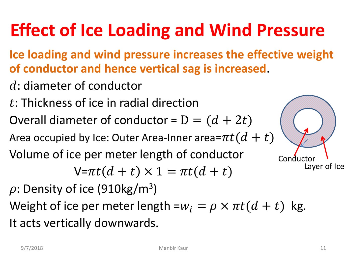
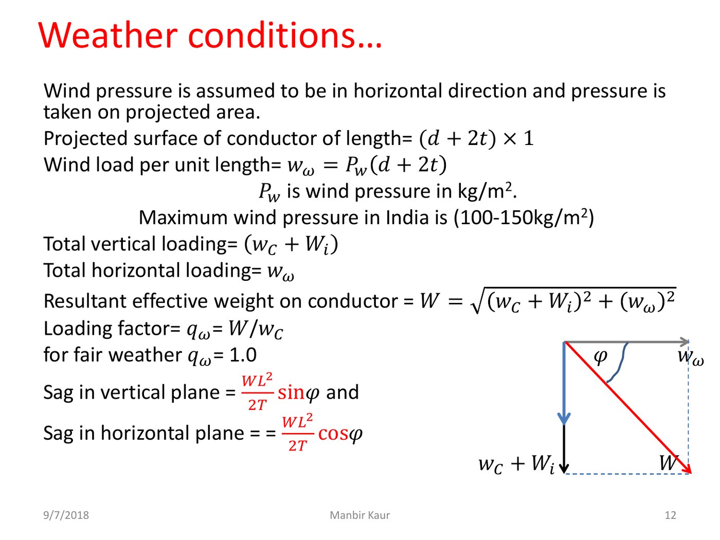
Ice adds weight straight down. Wind pushes sideways. The conductor hangs along the resultant, so its sag is measured in that tilted direction and only part of it is vertical.

Ice weight. Ice forms an annulus around the conductor: outer diameter = d + 2t, inner = d. Area = π[(d+2t)² − d²]/4, times ice density, gives kg/m to add to the bare conductor weight.
Wind force. Wind pressure acts on the projected area, and with ice that area is (d + 2t) per metre of span — not d. So w_wind = pressure × (d + 2t).
Resultant. ω_r = √[(ω + ω_ice)² + ω_wind²], and it hangs at angle θ = tan⁻¹(w_wind/(ω + ω_ice)) from vertical.
Slant sag and its parts. S = ω_rL²/8T along the resultant. Vertical component = S cos θ, horizontal swing = S sin θ.
Cross-arm height. clearance + vertical sag + insulator string length (1.63 m here) — the string hangs below the cross-arm, so it adds.

Target answers: 8.14 m maximum sag, 1.78 m wind displacement, 17.27 m cross-arm height. Note the tensile strength is given in kg/cm², so multiply by the conductor's cross-sectional area to get T in kg.

Q20 · supports at different heights, vertex outside the span

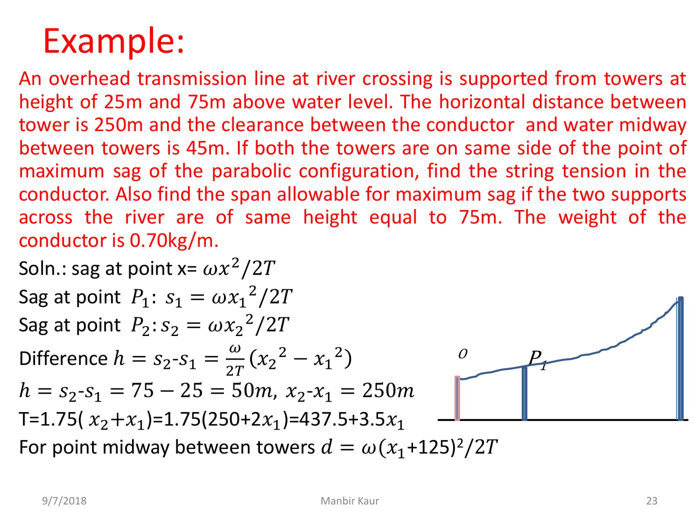
River crossing: 300 m span, towers 30 m and 85 m above water, both on the same side of the lowest point, ω = 1 kg/m, clearance 50 m at the mid-span point P. Find the tension.

measure x from the (imaginary) lowest point O; y = ωx²/2T

let x₁ = O to the 30 m tower, so x₁+300 = O to the 85 m tower

height difference: [(x₁+300)² − x₁²] / 2T = 55

→ (600x₁ + 90000) / 2T = 55

at mid-span, x = x₁+150, rise above the 30 m tower = 20

→ (300x₁ + 22500) / 2T = 20

divide: ratio = 2.75 → 225x₁ = 28125 → x₁ = 125 m

2T = (300·125 + 22500)/20 = 3000

T = 1500 kg — matches the sheet.

Trap · "same side of the point of maximum sag"

That phrase is the whole question. It means the lowest point of the curve lies outside the span — the conductor is still rising across the entire crossing. Both x₁ and x₂ are therefore positive and measured the same way, which is what makes the two equations above solvable. If you assume the vertex sits between the towers you will get a negative distance and no answer.

Trap · factor of safety divides, it never multiplies

Working tension = ultimate strength ÷ factor of safety. Multiplying gives a conductor four times too strong and a sag four times too small — and a suspiciously short tower.

Trap · the insulator string counts

Q19 gives a 1.63 m string for a reason. The conductor hangs at the bottom of it, so the cross-arm must sit that much higher than the conductor's own required height.

Q18Minimum support height T = strength/FoS, S = ωl²/2T with l = 150, then add clearance. 13 m — reproduced exactly

Q19Sag with ice and wind Ice annulus, wind on (d+2t), resultant, then resolve. Add the 1.63 m string. 8.13 m ✓ · 17.26 m ✓1.78 m → 6.37 m

Q20River crossing tension Vertex outside the span; two equations in x₁ and T, divide to eliminate T. 1500 kg — reproduced exactly

Q19's two panels. Left: the ice annulus, drawn to scale — 1.5 cm conductor inside 1.25 cm of ice gives the 4.0 cm the wind actually pushes on. Right: the load triangle, and the three different lengths people confuse — slant sag 10.33 m, vertical sag 8.13 m (the one asked for), wind displacement 6.37 m.

Q20 to scale, from its own solution. Both towers sit on the same limb of the parabola, so the lowest point O is 125 m outside the span and 24.79 m above the water. x₁ and x₂ are measured from O, not from the left tower — that datum is the whole difficulty. Solving gives the printed T = 1500 kg.

Unit 3, as she taught it

Four slides: the two support cases, and what ice and wind do to the load.

Unit 3, as she taught it — slide 11 — **Ice loading.** Overall diameter becomes d + 2t and the ice weight is ρ·π·t(d + t) per metre, acting straight down with the conductor's own weight. (U3 slide 11)

Unit 3, as she taught it — slide 12 — **Wind and ice together.** Wind acts horizontally on the projected area (d + 2t)×1, so the resultant is the hypotenuse — and the sag you compute is in the *slant* plane. (U3 slide 12)

Unit 3, as she taught it — slide 23 — **The river-crossing example** with unequal support heights, worked end to end. Q20 is the same shape. (U3 slide 23)

Sheet 6 · Q21–Q24 Unit 5

Why the bottom insulator always fails first

A string of identical discs does not share voltage equally, because stray capacitance to the tower steals current. Four problems on quantifying and fixing that.

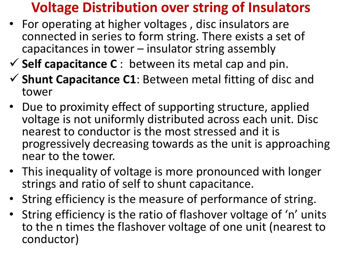
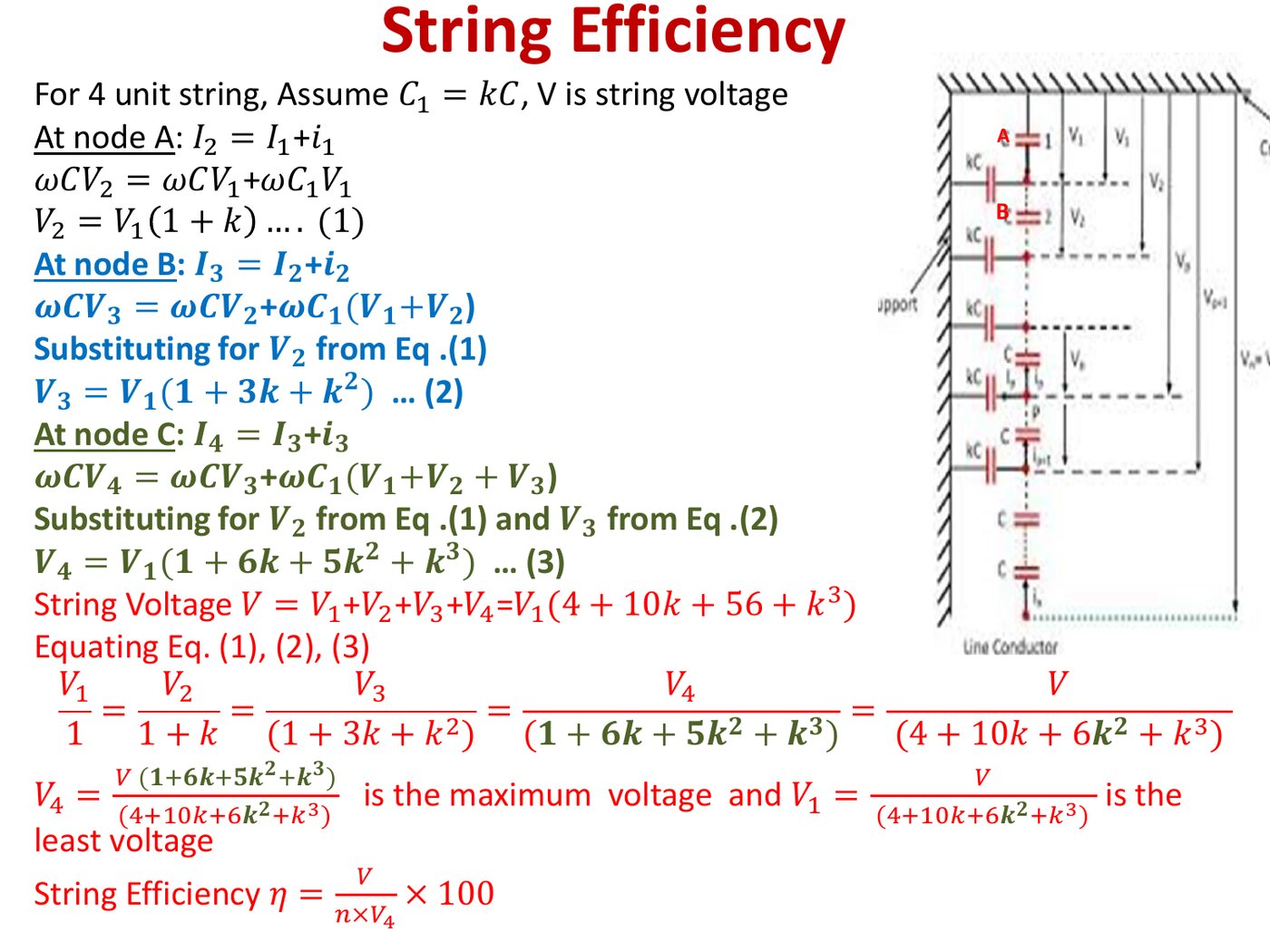
Stack four identical insulator discs and you would expect each to take a quarter of the voltage. They do not. Each metal link between discs also has a small capacitance to the earthed tower, and that stray path draws off current. So the disc nearest the line carries the most current — and the most voltage — and is the one that flashes over. Every question on this sheet follows from that single asymmetry.

Write k = C₁/C for the ratio of stray capacitance to disc self-capacitance. Apply Kirchhoff at each link and the voltages come out as a fixed pattern, counting from the top (tower end) downward:

Voltage across each disc, top-down V₂ = V₁(1 + k) · V₃ = V₁(1 + 3k + k²) · V₄ = V₁(1 + 6k + 5k² + k³)

String efficiency η = Vn × V_bottom × 100 %

kstray-to-self capacitance ratio; "1/10th of self" means k = 0.1
Vtotal voltage across the whole string
nnumber of discs
V_bottomthe most stressed disc — the one nearest the line

Q21 · four discs, k = 0.1, 132 kV to earth

V₁ = V₁

V₂ = 1.100 V₁

V₃ = 1 + 0.3 + 0.01 = 1.310 V₁

V₄ = 1 + 0.6 + 0.05 + 0.001 = 1.651 V₁

sum = 5.061 V₁ = 132 kV → V₁ = 26.08 kV

V₂ = 28.69 V₃ = 34.17 V₄ = 43.06 kV

η = 132 / (4 × 43.06) = 76.63 %

26.08 · 28.69 · 34.17 · 43.06 kV, η = 76.6% — all five match the sheet.

Q22 · the √2 that decides the answer

Three discs, k = 0.15, and "the maximum peak voltage per unit is not to exceed 35 kV". Find the greatest working voltage and the string efficiency.

the formulas are rms; the limit is peak — convert it first

V₃(rms) = 35 / √2 = 24.75 kV

V₃ = V₁(1 + 0.45 + 0.0225) = 1.4725 V₁

V₁ = 24.75 / 1.4725 = 16.81 kV

V₂ = 16.81 × 1.15 = 19.33 kV

V = 16.81 + 19.33 + 24.75 = 60.89 kV

η = 60.89 / (3 × 24.75) = 82.0 %

60.89 kV, η = 82% — matches. Skip the √2 and you get 86.1 kV, which is the classic wrong answer to this question.

Q23 & Q24: the guard ring

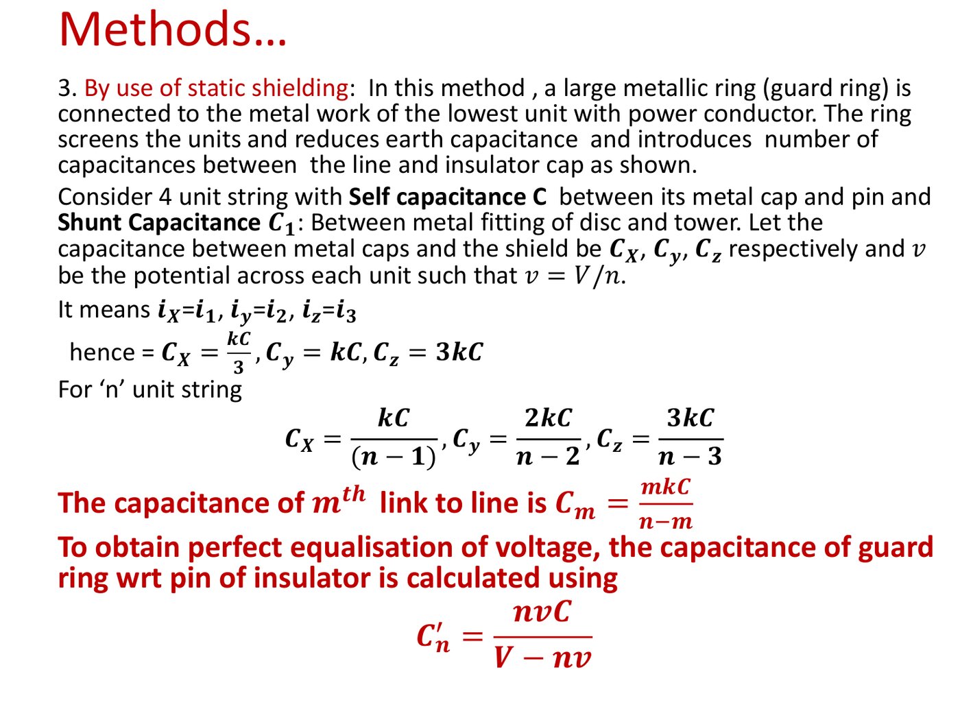
The fix for unequal sharing is a guard ring — a metal ring around the bottom disc that adds deliberate capacitance to the line, feeding current back in to cancel what the stray path to earth stole. Design it right and every disc takes an equal share.

Guard-ring condition for exactly uniform distribution n C = (k − n) C_n → C_n = n Ck − n

nlink number, counted from the top
khere the number of discs — not the capacitance ratio. Wadhwa reuses the letter on p200; watch it
C_nrequired capacitance from the guard ring to link n

Q23 · six discs, so k = 6:
n=1 → C/5 = 0.2C   n=2 → 2C/4 = 0.5C   n=3 → 3C/3 = C
n=4 → 4C/2 = 2C   n=5 → 5C/1 = 5C

0.2C · 0.5C · C · 2C · 5C — matches the sheet exactly. Q24 is the partial version: a ring that only improves the bottom disc, so solve the node equations with both a 0.2C path to earth and a 0.15C (0.3C at the bottom) path to line, and report the resulting η = 90.27%.

Trap · is the given voltage across the string, or line-to-line?

Q21 says "between the line conductor and the earth", which is already the voltage across one string — use 132 kV directly. Unit 5's Example 2 says "a 33 kV line", which is line-to-line, so it divides by √3 first. Same formulas, different starting number, and the question's wording is the only clue.

Trap · count from the top, stress at the bottom

V₁ is the disc at the tower and is the smallest. The efficiency denominator uses the largest, V_n, nearest the line. Getting the direction backwards produces an efficiency above 100%, which is your signal to flip.

Trap · two different k's in one sheet

In Q21–Q22, k is the capacitance ratio C₁/C. In the guard-ring formula of Q23, k is the number of discs. They are unrelated quantities that happen to share a letter in the source material.

Q21Four discs, voltage distribution k = 0.1, sum = 5.061 V₁ = 132 kV. 26.08 / 28.69 / 34.17 / 43.06 kV, 76.6% — all reproduced

Q22Greatest working voltage Convert the 35 kV peak limit to 24.75 kV rms first. 60.89 kV, 82% — reproduced exactly

Q23Guard-ring capacitances C_n = nC/(6−n) for n = 1…5. 0.2C / 0.5C / C / 2C / 5C — reproduced exactly

Q24Efficiency with a partial guard ring Node equations with 0.2C to earth and 0.15C/0.3C to line. 90.27 % is the no-guard-ring value → 97.31 %

Q24's network. Each pin has 0.2C stealing current to the earthed tower, which is why the bottom unit works hardest. The guard ring raises the bottom pin's capacitance to the line from 0.15C to 0.30C and hands that current back. With the ring the efficiency is 97.31 %; the sheet's 90.27 % is the figure without it.

Unit 5, as she taught it

Three slides cover Sheet 6 completely.

Unit 5, as she taught it — slide 24 — **String efficiency, derived for four units.** η = V/(n·V₁) with V₁ the *bottom* unit — the most stressed one, nearest the conductor. (U5 slide 24)

Unit 5, as she taught it — slide 27 — **The guard ring.** Q23/Q24's condition: the ring's capacitance to the nth pin must supply the extra current the shunt capacitance steals, C′ₙ = n·v·C/(V − n·v). (U5 slide 27)

Sheet 7 · Q25–Q30 Unit 6

Cables: a cylinder of stressed insulation

Bury the line and the geometry becomes coaxial. Six problems on leakage, electric stress, grading, and the capacitance of a three-core cable.

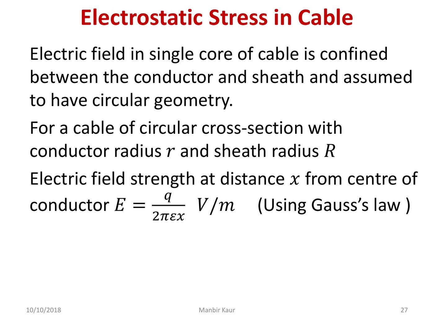
A single-core cable is a conductor of radius r inside a sheath of radius R, with insulation between. Every formula on this sheet is a coaxial-cylinder result, and they all contain ln(R/r). What makes cables interesting is that the electric stress is not uniform: it is highest right at the conductor surface and falls outward. The insulation nearest the conductor is therefore doing all the suffering, and most of Unit 6 is about that unfairness.

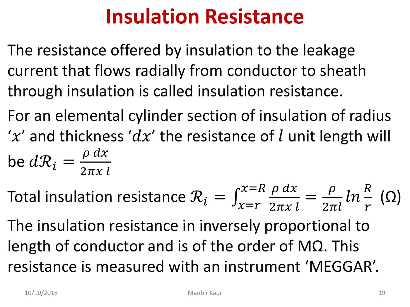
Insulation resistance — leakage across the insulation R_ins = ρ2π l ln Rr Ω

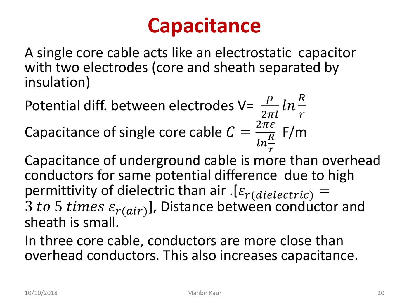
Capacitance C = 2π εln ( R / r ) F/m

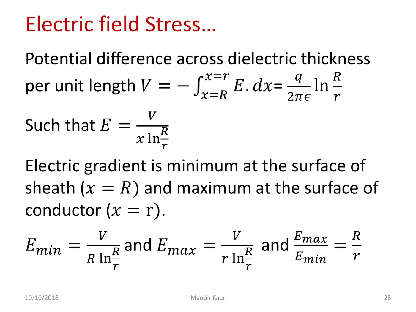
Electric stress at radius x g(x) = Vx · ln ( R / r )

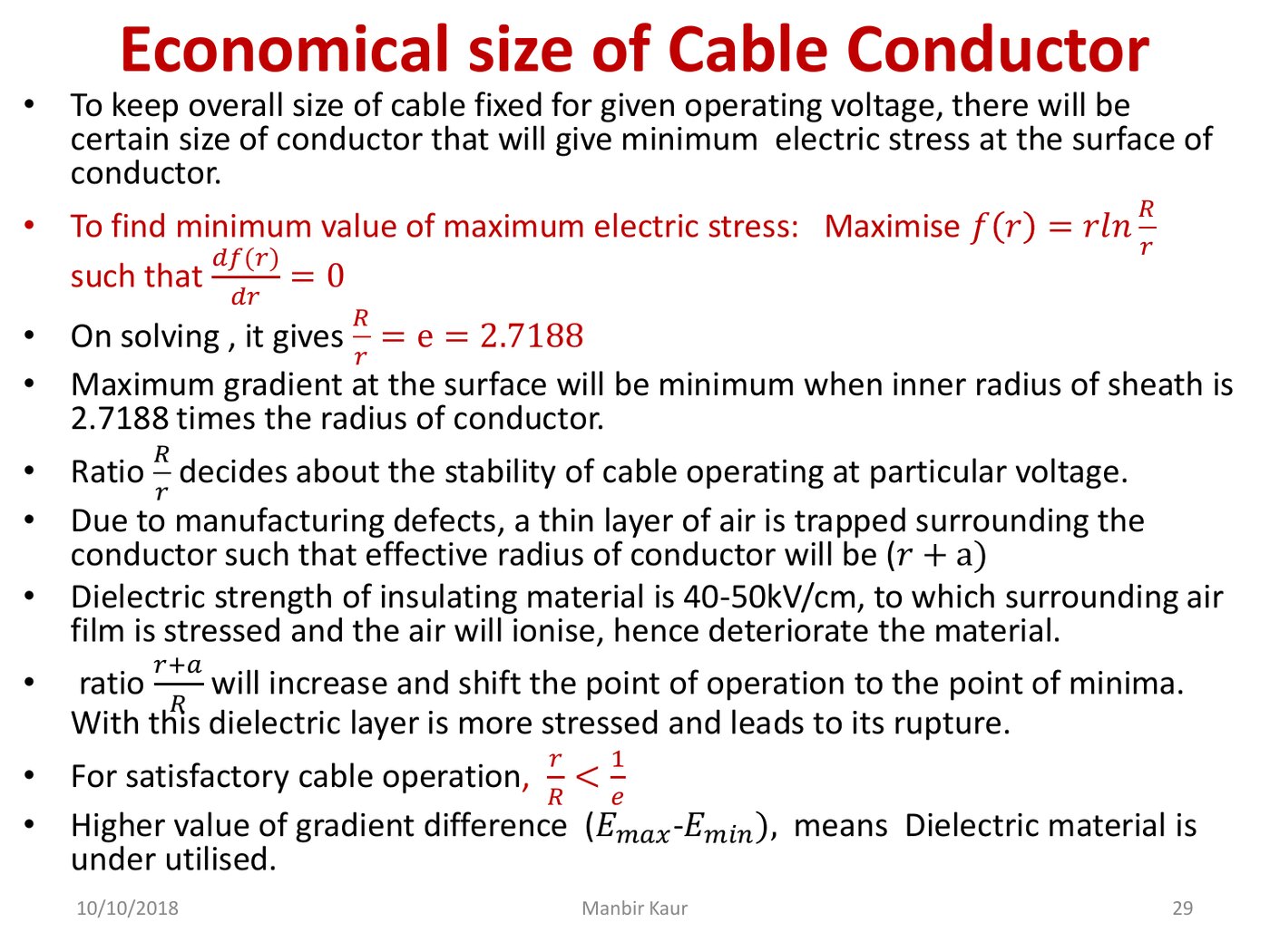
Most economical conductor size ln Rr = 1 → R = e·r → r = Vg_max

Why the "most economical size" formula looks like magic

Stress is worst at the conductor surface, where g_max = V/(r ln(R/r)). Hold the voltage fixed and ask which r makes that smallest: differentiate r·ln(R/r) with respect to r, set it to zero, and you get ln(R/r) = 1 — that is, R = e·r ≈ 2.718 r. Substituting back, g_max = V/r, so the conductor radius you want is simply V/g_max. A cable can be too thin for its voltage: a hair-thin conductor concentrates the field and punches through insulation that a fatter one would survive.

Q26 · both answers hinge on peak voltage

275 kV three-phase system, maximum stress 15 kV/mm. Find the overall diameter and the most economical conductor diameter.

phase voltage, then peak — stress limits are peak limits

V = 275/√3 × √2 = 224.5 kV

r = V/g_max = 224.5/15 = 14.97 mm

conductor diameter = 29.9 mm

R = e·r = 2.718 × 14.97 = 40.7 mm

overall diameter = 81.3 mm

81.3 mm and 29.9 mm — both match. Use rms and you get 21 mm and 58 mm, and nothing agrees.

Q29 · two dielectric layers

Conductor 10 mm diameter, two 10 mm layers, ε_r = 3 then 2.5, 60 kV across. Find the stress at the conductor surface.

r = 5, r₁ = 15, r₂ = 25 mm

D is continuous, so ε·g is continuous; add the layer voltages

D = (1/3)ln(15/5) + (1/2.5)ln(25/15)

= 0.3662 + 0.2043 = 0.5705

g = V / (ε_r1 · r · D)

= 60 / (3 × 5 × 0.5705)

7.01 kV/mm — matches the sheet.

Q30: grading, which is Q29 run in reverse

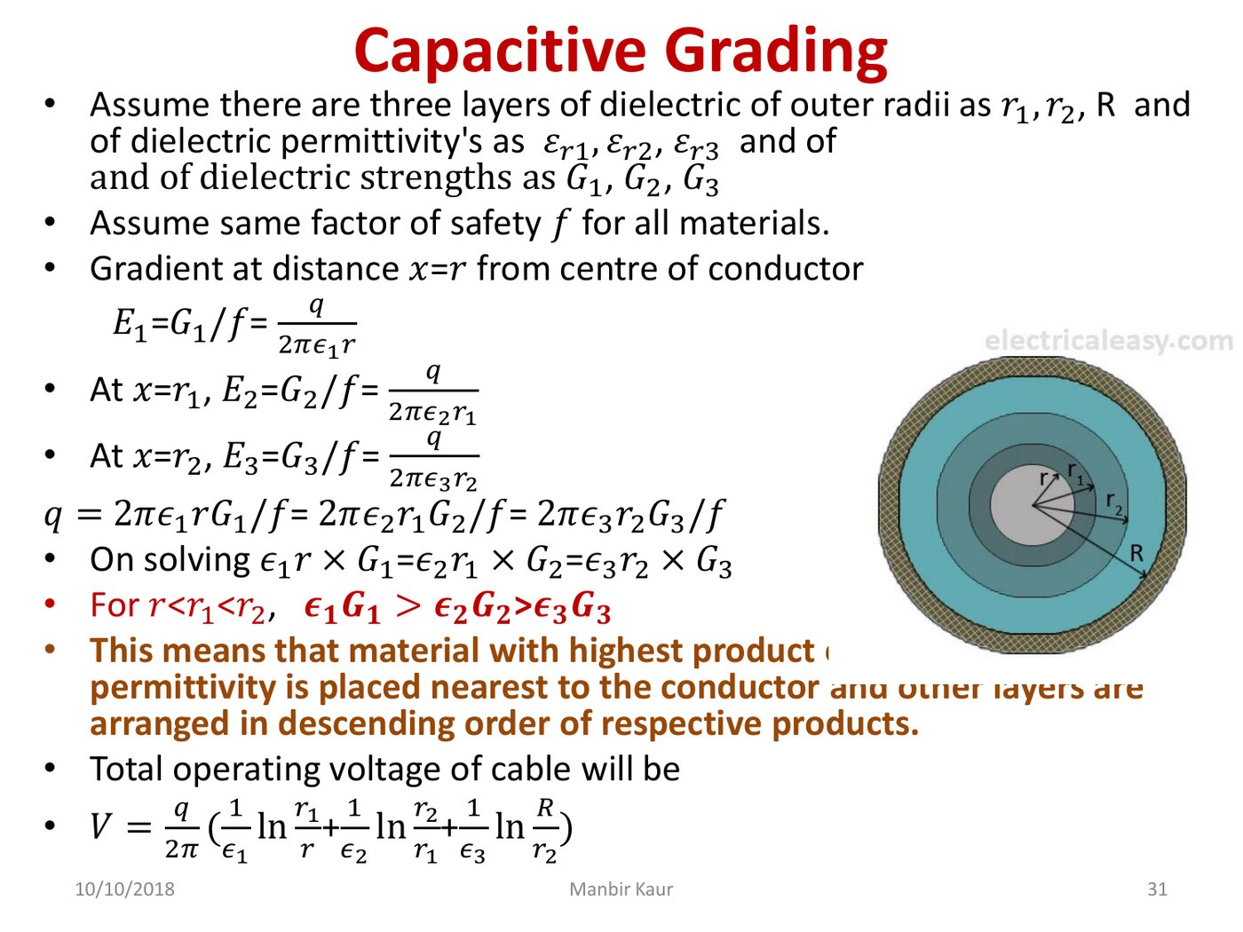
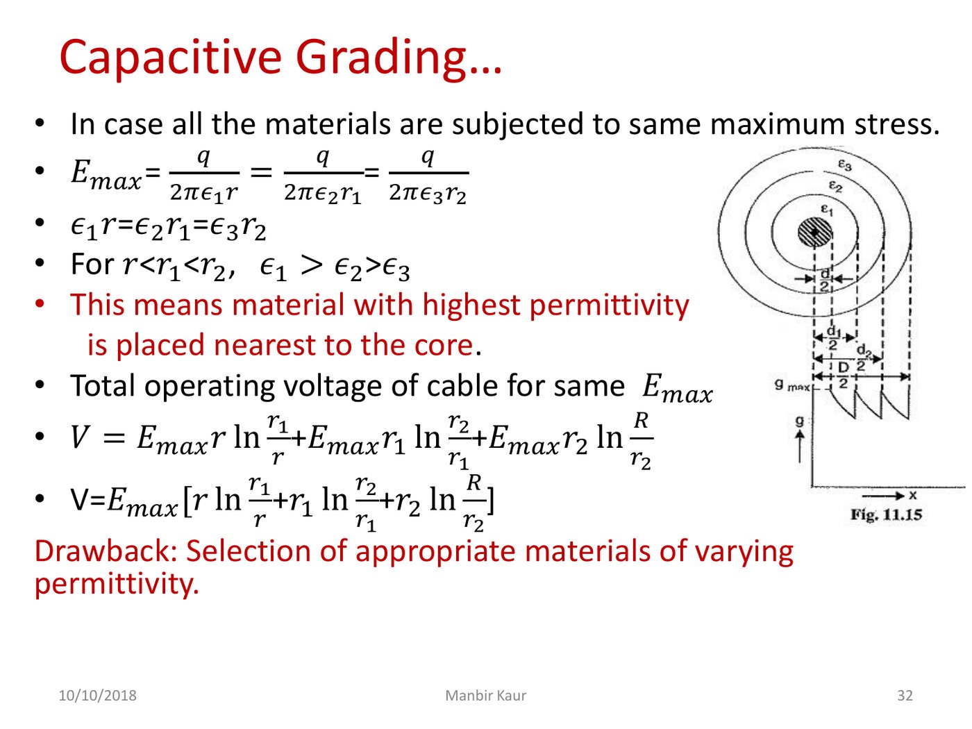
Grading means choosing layers so that each material sits exactly at its own maximum permissible stress — no material wasted, none over-stressed. The trick is that ε_r·g·x is the same constant everywhere in the cable, so one product fixes every boundary radius.

Fix the constant at the conductor: K = ε₁g₁r = 5 × 3.8 × 10 = 190.
Find each boundary from that same K: r₁ = K/(ε₂g₂) = 190/(4×2.6) = 18.27 mm, then r₂ = K/(ε₃g₃) = 190/(3×2) = 31.67 mm.
Add up the layer voltages: V = (K/ε₁)ln(r₁/r) + (K/ε₂)ln(r₂/r₁) + (K/ε₃)ln(R/r₂) — the first two give 22.9 + 26.2 = 49.1 kV of the 66 kV.
Solve for R from what's left: 63.33·ln(R/31.67) = 16.94 → R = 41.4 mm.

sheath diameter 82.8 mm — matches the sheet.

Q27 & Q28: three-core cable capacitance

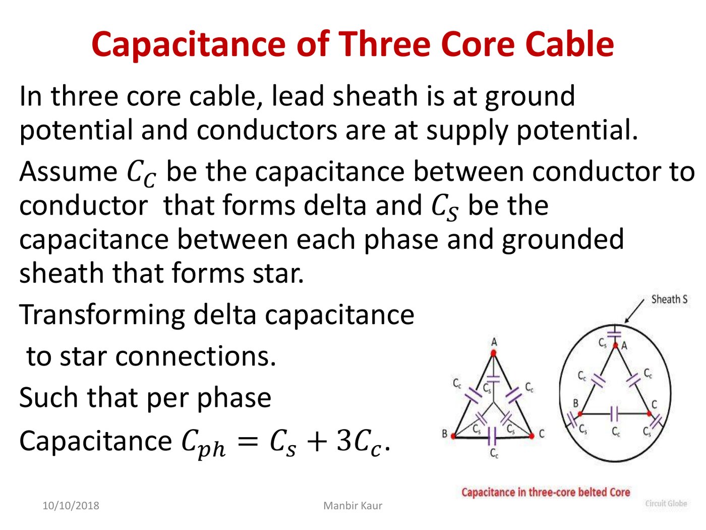
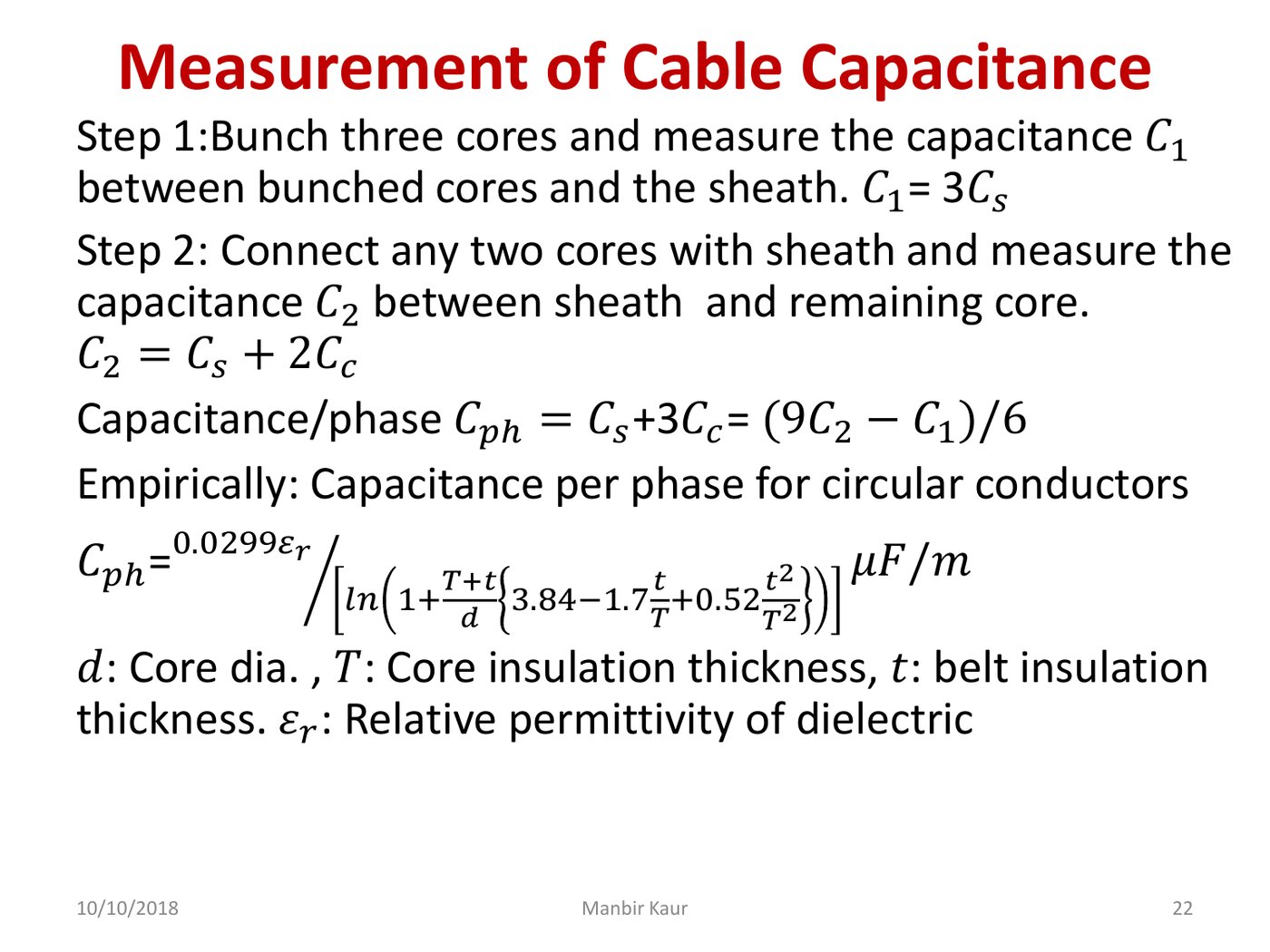
Three cores in one sheath have two kinds of capacitance: core-to-sheath (C_s) and core-to-core (C_c). You cannot measure either directly, so you make two accessible measurements and solve. Convert to the per-phase value C_ph = C_s + 3C_c, then everything else follows.

Q28 · from the two measurements
all three cores bunched vs sheath = 3Cs = 0.625 → Cs = 0.2083 µF/km
one core vs the other two + sheath = Cs + 2Cc = 0.4 → Cc = 0.0958
 
(a) between two cores = (Cs + 3Cc)/2 = 0.248 µF/km ✓
(b) two bunched vs the third = ⅔(Cs + 3Cc) = 0.331 µF/km ✓
(c) Cph = 0.4958 → I = 2πf Cph Vph = 0.899 A ✓

Q27 is the short version: a measured 2 µF between any two cores means C_ph = 2 × 2 = 4 µF, so I = 2πf C_ph(11000/√3) = 7.98 A and Q = 3V_phI = 152 kVAr. Both match.

Trap · two different resistances live in a cable

The conductor's own resistance goes along the cable and falls as area rises. Insulation resistance goes across the insulation and falls as the cable gets longer — twice the length is twice the leakage path in parallel. In Q25 the 5 km divides, it does not multiply.

Trap · stress limits are peak, voltages are usually rms

Q26 needs 275/√3 × √2. Q30 states its stresses as rms and gives 66 kV to earth, so no √2 is needed there — read each question's own wording rather than applying a habit.

Trap · don't reuse a C₁/C₂ formula whose convention you can't pin

Unit 6 quotes C_ph = (9C₂ − C₁)/6 for the measurement problem. Feed Q28's numbers into it and you get 0.871, not the 0.4958 that reproduces the printed answers — its C₁ and C₂ mean different measurements than Q28's (i) and (ii). Derive C_s and C_c from whatever the question actually measured, as above, and you will not get caught.

Q25Resistivity from insulation resistance ρ = R_ins · 2πl / ln(R/r), with l = 5000 m. 13.72×10³ MΩ·m — reproduced as 13.71

Q26Overall and economical diameter Peak phase voltage 224.5 kV; r = V/g, R = e·r. 81.32 mm, 29.92 mm — both reproduced

Q27Charging current and kVAr C_ph = 2 × (measured core-to-core) = 4 µF. 8 A, 152.4 kVAr — reproduced as 7.98 / 152

Q28Three-core capacitance from two tests 3C_s and C_s+2C_c → solve, then combine. 0.248 / 0.33 µF/km, 0.899 A — all reproduced

Q29Stress with two dielectrics g = V/(ε_r1·r·Σ(1/ε)ln ratios). 7.01 kV/mm — reproduced exactly

Q30Minimum sheath diameter, graded cable K = εgr constant fixes every boundary; sum layer voltages to 66 kV. 82.8 mm — reproduced exactly

What grading actually does, on Q30's numbers. The dashed curve is one dielectric: its stress peaks at 4.65 kV/mm at the core, above what the innermost material can take. Graded, each layer starts at its own rating and falls as 1/x, jumping back up at each boundary because D = εE is continuous while ε drops. The layer radii come out at 18.27 and 31.67 mm, and the sheath at 82.8 mm diameter — the printed answer.

Unit 6, as she taught it

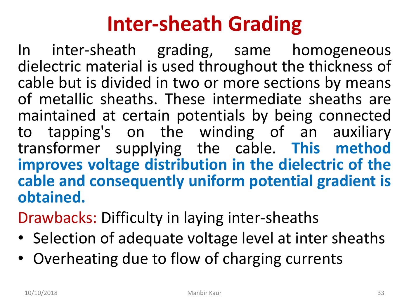
Eleven slides: resistance, capacitance, stress, economical size, and both grading methods.

Unit 6, as she taught it — slide 20 — **The cable as a coaxial capacitor.** C = 2πε/ln(R/r) per metre. Q25 and Q26 are this line. (U6 slide 20)

Unit 6, as she taught it — slide 21 — **Three-core belted cable.** C_s core-to-sheath and C_c core-to-core; the delta of C_c transforms to a star of 3C_c, giving C_ph = C_s + 3C_c. (U6 slide 21)

Unit 6, as she taught it — slide 22 — **The two measurements Q27/Q28 quote.** Bunch all three cores against the sheath → C₁ = 3C_s; two cores against sheath-plus-third → C₂ = C_s + 2C_c. Careful: the (9C₂ − C₁)/6 shortcut on this slide is written for *different* C₁, C₂ definitions and does not reproduce Q28's printed answer — derive C_s and C_c from the stated tests instead. (U6 slide 22)

Unit 6, as she taught it — slide 27 — **Electrostatic stress.** E(x) = q/2πεx, so the field is largest at the conductor surface and smallest at the sheath. (U6 slide 27)

Unit 6, as she taught it — slide 28 — **E_max and E_min.** E_max = V/(r·ln(R/r)), and E_max/E_min = R/r. Q26 is this solved for r. (U6 slide 28)

Unit 6, as she taught it — slide 29 — **Most economical conductor size.** Minimising E_max over r gives ln(R/r) = 1, i.e. R/r = e = 2.7183 — the 'magic' constant in Q29. (U6 slide 29)

Unit 6, as she taught it — slide 31 — **Capacitive grading.** Layers of decreasing permittivity outward, so the highest-ε material sits against the core. (U6 slide 31)

Unit 6, as she taught it — slide 32 — **Equal-stress grading.** With every layer at the same E_max, the total voltage is a sum of E_max·r_i·ln(r_i+1/r_i) terms. (U6 slide 32)

Unit 6, as she taught it — slide 33 — **Inter-sheath grading.** One dielectric, metallic sheaths held at intermediate potentials by an auxiliary transformer. (U6 slide 33)

Unit 6, as she taught it — slide 36 — **Optimum inter-sheath position.** r₁ = 1.76 r, and a single inter-sheath raises the permissible operating voltage by 33 % for the same overall size. (U6 slide 36)

Answers the sheet does not print Computed here

Ten numbers to check yourself against — and four the sheet gets wrong

Every problem on the seven sheets now has a number attached. These ten had nothing to check against, so each was derived twice, by different routes, before being written down.

Treat this table differently from the rest of the page. Elsewhere, "reproduced" means the method here regenerated a number your instructor printed — an independent check. Here there was nothing to check against, so what follows is our answer, and the confidence column is the honest uncertainty, not decoration. Where an assumption had to be made, it is named: if your lecturer's convention differs, the assumption is the line to change.

Q	Answer	How it was checked	Confidence
Q1	dc 2-wire is cheapest (1.00); best ac is 3-φ 3-wire (1.50)	All ten rows of her p48 table re-derived from v = P²ρl²/(WV²cos²θ); ranking holds for any power factor, since the smallest ac coefficient (1.5) already beats dc 3-wire's 1.25	High
Q2	P₂ = 2P₁cos²θ → +100 % at unity pf	Same algebra as her own p50 sample calculation, which also lands on 100 %. No pf is given in the question; at 0.9 it would be +62 %	Medium — rests on unity pf
Q3	1178 · 1512 · 1474 A; neutral 604 A	Phasor sum per phase, then power balance back out of the final phasors: 241.667 + 286.667 + 316.667 = 845.000 kW against the stated 845 kW	High
Q4	3-wire costs 0.3125 × the 2-wire (saves 68.75 %)	Derived twice — from currents, and from the volume formula — and lands on the 0.3125 already printed in her table. Absolute rupees are not obtainable: neither line length nor efficiency is given, and cost scales as L²·η/(1−η)	High on the ratio, none on absolute cost
Q6	j18.24 Ω per phase at 66 kV (0.1466 pu)	Convention validated by re-deriving Q5's four printed values first. Reading the wording literally — generator terminals to output terminals — would give 4.84 Ω, the transformer alone, which makes the generator data pointless	High on arithmetic, medium on wording
Q7	424.4 V (1.0611 pu ∠ +4.03°)	Same answer to five significant figures from an all-per-unit route and an all-ohms route referred to circuit C. Each transformer's pu reactance also agrees computed from either winding — the check that fails if the voltage bases are wrong	High
Q10	R_dc = 0.1093 Ω/km; R_ac = 0.120–0.125 Ω/km	Back-substitution recovers the input resistivity exactly. The conductor is real — 322 mm², 37 × 0.333 cm is AAC "Orchid", published R_dc(20 °C) 0.0897 vs our 0.0895	High on dc, medium on ac — see the note below
Q13	D = 1.48 m maximum spacing	Plug-back gives 31.400 Ω. Omitting the loop factor of 2 would give 218 m, physically absurd — so the factor is load-bearing, and 1.48 m sits right beside the sheet's own 1.5 m (Q14) and 1.8 m (Q17) spacings	High
Q16	12.62 nF/km/phase · I_c = 0.504 A/km · 192 kVAr/km	Geometry validated by reproducing Q12's printed 0.906 mH/km, the current convention by reproducing Q15's printed 0.226 A/km and 51.7 kVAr, and the bundle formula by her own 400 kV example on Unit 4 p18	High
Q17	0.2113 µF, rising to 0.2115 µF with ground	Not actually unverifiable: this exact question is worked on Unit 4 p16 with 0.2111 and 0.2114 printed. Ground formula also cross-checked against Wadhwa eq. 3.43	High

Q10 · the deck's 10–14 % skin effect is too big for this conductor

Unit 2 p10 says skin effect adds 10–14 %, and that is the band used above because it is what your course says. But published data for this conductor gives R_ac/R_dc ≈ 1.01 at 60 Hz, and her own worked example on p16 finds only 3.7 %. The 10–14 % figure is generic — it belongs to large-diameter conductors at higher frequency, not a 2.3 cm all-aluminium conductor at 50 Hz. Quote the deck's band in an exam; know that the physics disagrees.

Q4 · one assumption decides the whole answer

"Consumer's terminal voltage 220 V" has to mean line-to-neutral, so the three-wire outers sit 440 V apart. Her Assignment-1 slide (Unit 1 p49) says exactly that — "220V (line to neutral)". Read 220 V as the outer-to-outer voltage instead and the ratio inverts to 1.25, making the three-wire system 25 % more expensive. State the reading you used.

Four errors in the tutorial sheet

Where	Printed	Should be	How we know
Q11	1.2947 H/km	1.2947 mH/km	Unit typo only — the digits are right
Q8	Rs 24 359	Rs 24 357	Rounding in the sheet; every other value in Q8 reproduces
Q19 (ii)	1.78 m	6.37 m	Parts (i) and (iii) of the same question pin T = 2209 kg and w_v = 2.299 kg/m; with those fixed, 1.78 m needs a wind pressure of 12.6 kg/m², not the stated 45. Nine alternative conventions were tried and none lands near 1.78. It cannot be insulator swing either — that is 1.00 m, and 1.78 m exceeds the 1.63 m string length
Q24	90.27 %	97.31 %	90.27 % is the efficiency without the guard ring, reproduced to five significant figures (90.269 %). It is Wadhwa Example 8.2 with 0.1C changed to 0.15C, and the sheet kept the "before" number while the question asks for the "after"

Three errors in Unit 1's comparison table

Eight of the ten rows on slide p48 reproduce exactly, and the scaling identity col B = col A × (V_cc/V_ce)² confirms those eight to three decimals. It fails on precisely the two two-phase rows, which is what identifies them as slide errors rather than a misunderstanding on our side. All three were checked against the raw PDF text, so they are in the slide, not in the transcription.

Row	Printed	Should be
2-φ 3-wire, conductor–conductor column	2	2.914
2-φ 4-wire, conductor–conductor column	2.194	2.0
1-φ 2-wire mid-point earthed, volume column	2.5Al	2Al — the printed ratio 0.5 is only reachable with 2Al

None of this changes Q1's answer — dc two-wire still wins, and three-phase three-wire is still the best ac system, which is the conclusion her own slide states.

Recap

The whole toolkit on one screen

If you remember nothing else, remember these — and which constant goes with which.

Constants worth memorising: 2πε₀ = 5.5626×10⁻¹¹, πε₀ = 2.7813×10⁻¹¹, 2π(50) = 314.16.
Quantity	Formula	Watch for
Conductor volume	P²ρl² / (W V² cos²θ)	Which V the question holds fixed
Per unit	Z_pu = Z_Ω·MVA_b / kV_b²	Base MVA on top when changing base
Kelvin's law	rate × variable capital = annual loss cost	Fixed cost never enters
Inductance	2×10⁻⁷ ln(D_eq/D_s) H/m	D_s = 0.7788r
Capacitance, 3-φ	2πε₀ / ln(D_eq/r) F/m	True r, not 0.7788r
Capacitance, 1-φ	πε₀ / ln(D/r) F/m	π, not 2π — it's between two wires
Equivalent spacing	³√(D₁₂D₂₃D₃₁)	Transposed lines only
Bundle, 2 sub-conductors	√(r′d) for L · √(rd) for C	Same d, different radius
Sag	ωL²/8T, or ωl²/2T with half-span	T = strength ÷ FoS
String, disc n from top	V₂=V₁(1+k), V₃=V₁(1+3k+k²)	Bottom disc is the stressed one
String efficiency	V / (n·V_bottom) × 100	Over 100% means you flipped it
Guard ring	C_n = nC/(k−n), k = disc count	Different k from the ratio k
Insulation resistance	(ρ/2πl) ln(R/r)	Longer cable → lower resistance
Cable stress	g(x) = V / (x ln(R/r))	Peak, not rms
Economical cable	ln(R/r) = 1, r = V/g_max	R = 2.718 r
Graded cable	ε·g·x = constant	One constant fixes all boundaries
3-core cable	C_ph = C_s + 3C_c	Derive C_s, C_c from the actual test